Page 33 - MATLAB an introduction with applications

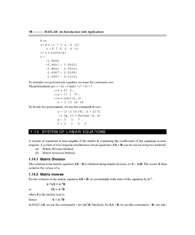
18 ——— MATLAB: An Introduction with Applications

% or
>> x = [5 7 0 2 –6 10]
x = 5 7 0 2 –6 10
>> r = roots(x)
r =
–1.8652
–0.4641 + 1.0832i
–0.4641 – 1.0832i
0.6967 + 0.5355i
0.6967 – 0.5355i
To multiply two polynomials together, we enter the command conv.
2
The polynomials are: x = 2x + 5 and y = x + 3x + 7
>>x = [2 5];
>>y = [1 3 7];
>>z = conv(x, y)
z = 2 11 29 35
To divide two polynomials, we use the command deconv.

z = [2 11 29 35]; x = [2 5]
>> [g, t] = deconv (z, x)
g = 1 3 7
t = 0 0 0 0

1.14 SYSTEM OF LINEAR EQUATIONS

A system of equations is non-singular if the matrix A containing the coefficients of the equations is non-
singular. A system of non-singular simultaneous linear equations (AX = B) can be solved using two methods:
(a) Matrix Division Method.
(b) Matrix Inversion Method.

1.14.1 Matrix Division
The solution to the matrix equation AX = B is obtained using matrix division, or X = A/B. The vector X then
contains the values of x.

1.14.2 Matrix Inverse
–1
For the solution of the matrix equation AX = B, we premultiply both sides of the equation by A .
–1
–1
A AX = A B
–1
or IX = A B
where I is the identity matrix.
–1
Hence X = A B
*
In MATLAB, we use the command x = inv (A) B. Similarly, for XA = B, we use the command x = B * inv (A).

F:\Final Book\Sanjay\IIIrd Printout\Dt. 10-03-09