Page 383 - MATLAB an introduction with applications

368 ——— MATLAB: An Introduction with Applications

0.850000 0.016805 0.358166
0.900000 0.019458 0.401200
0.950000 0.022246 0.446618
1.000000 0.025144 0.494409

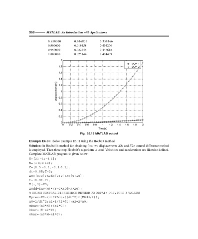
2
DOF-1
1.8 DOF-2

1.6
1.4
Displacement(m) 0.8
1.2
1

0.6
0.4

0.2
0
0 0.2 0.4 0.6 0.8 1 1.2 1.4 1.6 1.8 2
Time(s)
Fig. E6.13 MATLAB output

Example E6.14: Solve Example E6.11 using the Houbolt method.
Solution: In Houbolt’s method for obtaining first two displacements X∆t and X2t, central difference method
is employed. Then three step Houbolt’s algorithm is used. Velocities and accelerations are likewise defined.
Complete MATLAB program is given below:
K=[21 –1;–1 1];
M=[1 0;0 10];
C=[0.5 –0.1;–0.1 0.1];
dt=0.05;T=2;
X0=[0;0];X0d=[0;0];F=[0;10];
t=[0:dt:T];
X(:,2)=X0;
X0dd=inv(M)*(F–C*X0d–K*X0);
% USING CENTRAL DIFFERENCE METHOD TO OBTAIN PREVIOUS 3 VALUES
Xprev=X0–(dt*X0d)+((dt^2)*(X0dd/2));
a0=1/dt^2;a1=1/(2*dt);a2=2*a0;
mbar=(a0*M)+(a1*C);
kbar=(K–a2*M);
cbar=(a0*M–a1*C);