Page 385 - MATLAB an introduction with applications

370 ——— MATLAB: An Introduction with Applications

0.350000 0.001161 0.061114
0.400000 0.001782 0.079784
0.450000 0.002588 0.100924
0.500000 0.003595 0.124528
0.550000 0.004817 0.150590

0.600000 0.006260 0.179102
0.650000 0.007927 0.210055
0.700000 0.009814 0.243443
0.750000 0.011912 0.279255
0.800000 0.014208 0.317483
0.850000 0.016686 0.358115
0.900000 0.019325 0.401142
0.950000 0.022104 0.446553
1.000000 0.025000 0.494334

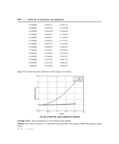
Figure E6.14 shows the plot of histories of two degrees of freedom.

2.5
DOF-1
DOF-2
2

1.5
Displacement(m) 0.5 1

0

–0.5
0 0.5 1 1.5 2 2.5
Time(s)
Fig. E6.14 MATLAB output (Houbolt’s method)
Example E6.15: Solve Example E6.11 by the Wilson Theta method.
Solution: Here, theta is chosen as 1.4 and followed the algorithm. The complete MATLAB program is given
below:

K=[21 –1;–1 1];