Page 388 - MATLAB an introduction with applications

Direct Numerical Integration Methods ——— 373

2
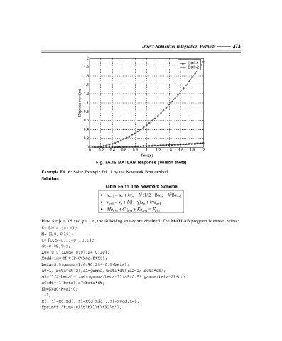
DOF-1
1.8 DOF-2
1.6

1.4
Displacement(m) 0.8 1
1.2

0.6

0.4
0.2

0
0 0.2 0.4 0.6 0.8 1 1.2 1.4 1.6 1.8 2
Time(s)
Fig. E6.15 MATLAB response (Wilson theta)
Example E6.16: Solve Example E6.11 by the Newmark Beta method.
Solution:
Table E6.11 The Newmark Scheme
2
β
• u n+ 1 = u + hv + h 2 (1/ 2 −β )a + h a n+ 1
n
n
n
• v n+ 1 = v + h (1− γ )a + γ n+ 1
h a
n
n
• Ma n+ 1 + Cv n+ 1 + Ku n+ 1 = F n+ 1
Here for β = 0.5 and γ = 1/6, the following values are obtained. The MATLAB program is shown below:
K= [21 –1;–1 1];
M= [1 0; 0 10];
C= [0.5 –0.1;–0.1 0.1];
dt=0.05;T=2;
X0=[0;0];X0d=[0;0];F=[0;10];
X0dd=inv(M)*(F–C*X0d–K*X0);
beta=0.5;gamma=1/6;%0.25*(0.5+beta);
a0=1/(beta*dt^2);a1=gamma/(beta*dt);a2=1/(beta*dt);
a3=(1/2*beta)–1;a4=(gamma/beta–1);a5=0.5*(gamma/beta–2)*dt;
a6=dt*(1–beta);a7=beta*dt;
Kb=K+a0*M+a1*C;
i=1;
X(:,1)=X0;Xd(:,1)=X0d;Xdd(:,1)=X0dd;t=0;
fprintf(‘time(s)\t\tX1\t\tX2\n’);