Page 151 - MATLAB Recipes for Earth Sciences

6.10 Adaptive Filtering 145

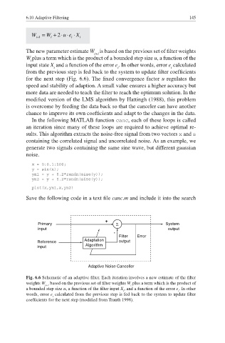
The new parameter estimate W is based on the previous set of fi lter weights
i+1
W plus a term which is the product of a bounded step size u, a function of the
i
input state X and a function of the error e . In other words, error e calculated
i i i
from the previous step is fed back to the system to update fi lter coeffi cients

for the next step (Fig. 6.6). The fixed convergence factor u regulates the
speed and stability of adaption. A small value ensures a higher accuracy but
more data are needed to teach the filter to reach the optimum solution. In the

modified version of the LMS algorithm by Hattingh (1988), this problem
is overcome by feeding the data back so that the canceler can have another

chance to improve its own coefficients and adapt to the changes in the data.
In the following MATLAB function canc, each of these loops is called
an iteration since many of these loops are required to achieve optimal re-
sults. This algorithm extracts the noise-free signal from two vectors x and s
containing the correlated signal and uncorrelated noise. As an example, we
generate two signals containing the same sine wave, but different gaussian
noise.

x = 0:0.1:100;
y = sin(x);
yn1 = y + 0.2*randn(size(y));
yn2 = y + 0.2*randn(size(y));
plot(x,yn1,x,yn2)

Save the following code in a text fi le canc.m and include it into the search

+
Primary Σ System
input output
-
Filter Error
Reference Adaptation output
Algorithm
input

Adaptive Noise Canceller

Fig. 6.6 Schematic of an adaptive filter. Each iteration involves a new estimate of the fi lter

weights W based on the previous set of fi lter weights W plus a term which is the product of
i+1 i
a bounded step size u, a function of the fi lter input X , and a function of the error e . In other
i i
words, error e calculated from the previous step is fed back to the system to update fi lter
i

coefficients for the next step (modified from Trauth 1998).