Page 150 - MATLAB Recipes for Earth Sciences

144 6 Signal Processing

steps required for the algorithm to converge close enough to an optimum
solution), misadjustment (measure of the amount by which the fi nal value
of the mean-squared error deviates from the minimum squared error of an

optimal filter, e.g., Wiener 1945, Kalman and Bucy 1961), and tracking (the

capability of the filter to work in a nonstationary environment, i.e., to track
changing statistical characteristics of the input signal) (Haykin 1991).
The simplicity of the least-mean-squares (LMS) algorithm, originally de-
veloped by Widrow and Hoff (1960), has made it the benchmark against
which other adaptive filtering algorithms are tested. For applications in earth

sciences, we use this filter to extract the noise from two signals S and X,
both containing the same signal s, but uncorrelated noise n and n (Hattingh
1 2
1988). As an example, consider a simple duplicate set of measurements on
the same material, e.g., two parallel stable isotope records from the same
foraminifera species. What you will expect are two time-series with N ele-
ments containing the same desired signal overlain by different uncorrelated
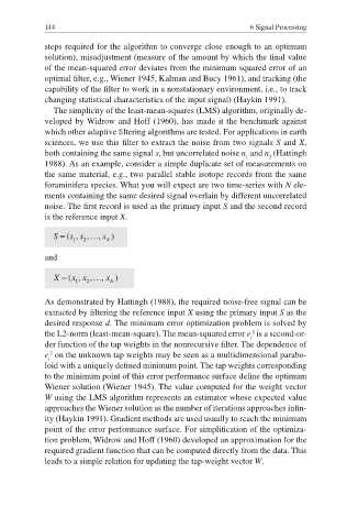
noise. The fi rst record is used as the primary input S and the second record
is the reference input X.

and

As demonstrated by Hattingh (1988), the required noise-free signal can be
extracted by fi ltering the reference input X using the primary input S as the
desired response d. The minimum error optimization problem is solved by
2
the L2-norm (least-mean-square). The mean-squared error e is a second-or-
i
der function of the tap weights in the nonrecursive filter. The dependence of

2
e on the unknown tap weights may be seen as a multidimensional parabo-
i

loid with a uniquely defined minimum point. The tap weights corresponding
to the minimum point of this error performance surface define the optimum

Wiener solution (Wiener 1945). The value computed for the weight vector
W using the LMS algorithm represents an estimator whose expected value
approaches the Wiener solution as the number of iterations approaches infi n-
ity (Haykin 1991). Gradient methods are used usually to reach the minimum
point of the error performance surface. For simplification of the optimiza-

tion problem, Widrow and Hoff (1960) developed an approximation for the
required gradient function that can be computed directly from the data. This
leads to a simple relation for updating the tap-weight vector W.