Page 145 - MATLAB Recipes for Earth Sciences

6.9 Filter Design 139

title('Magnitude Response')
1-interp1(f,magnitude,1/8)

ans =
0.6462
The phase response

phase = 180*angle(h)/pi;
f= w/(2*pi);

plot(f,unwrap(phase))
xlabel('Frequency'), ylabel('Phase in degrees')
title('Magnitude Response')

interp1(f,unwrap(phase),1/8) * 8/360
ans =
-5.0144

must again be corrected for causal indexing. The sampling interval was one,

the filter length is five, therefore we have to add (5-1)/2=2 to the phase shift
of -5.0144. This suggests a corrected phase shift of -3.0144, which is exactly
the delay seen on the plot.
plot(t,x11,t,y11), axis([30 40 -2 2])

The next chapter gives an introduction to the design of filters with a desired

frequency response. These filters can be used to amplify or suppress differ-
ent components of arbitrary signals.

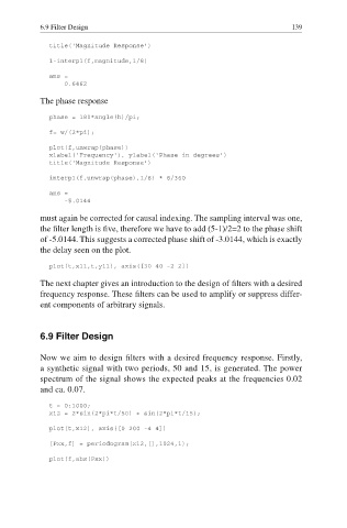
6.9 Filter Design

Now we aim to design filters with a desired frequency response. Firstly,
a synthetic signal with two periods, 50 and 15, is generated. The power
spectrum of the signal shows the expected peaks at the frequencies 0.02
and ca. 0.07.

t = 0:1000;
x12 = 2*sin(2*pi*t/50) + sin(2*pi*t/15);
plot(t,x12), axis([0 200 -4 4])

[Pxx,f] = periodogram(x12,[],1024,1);
plot(f,abs(Pxx))