Page 149 - MATLAB Recipes for Earth Sciences

6.10 Adaptive Filtering 143

6.10 Adaptive Filtering

The fi xed filters used in the previous chapters make the basic assumption
that the signal degradation is known and it does not change with time. In
most applications, however, an a priori knowledge of the signal and noise
statistical characteristics is usually not available. In addition, both the noise
level and the variance of the genuine signal can be highly nonstationary with
time, e.g., stable isotope records during the glacial-interglacial transition.

Fixed filters thus cannot be used in an nonstationary environment without a
knowledge of the signal-to-noise ratio.

In contrast, adaptive filters widely used in telecommunication industry

could help to overcome these problems. An adaptive filter is an inverse
modeling process, which iteratively adjusts its own coeffi cients automati-
cally without requiring any a priori knowledge of signal and noise. The

operation of an adaptive filter includes, (1) a filtering process, the purpose
of which is to produce an output in response to a sequence of data, and (2)
an adaptive process providing a mechanism for the adaptive control of the
filters weights (Haykin 1991).

In most practical applications, the adaptive process is oriented towards
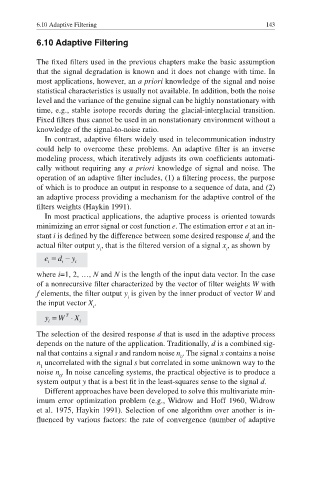
minimizing an error signal or cost function e. The estimation error e at an in-
stant i is defined by the difference between some desired response d and the

i
actual fi lter output y , that is the fi ltered version of a signal x , as shown by
i i

where i=1, 2, …, N and N is the length of the input data vector. In the case
of a nonrecursive fi lter characterized by the vector of fi lter weights W with
f elements, the fi lter output y is given by the inner product of vector W and
i
the input vector X .
i

The selection of the desired response d that is used in the adaptive process
depends on the nature of the application. Traditionally, d is a combined sig-
nal that contains a signal s and random noise n . The signal x contains a noise
0
n uncorrelated with the signal s but correlated in some unknown way to the
1
noise n . In noise canceling systems, the practical objective is to produce a
0

system output y that is a best fit in the least-squares sense to the signal d.
Different approaches have been developed to solve this multivariate min-
imum error optimization problem (e.g., Widrow and Hoff 1960, Widrow
et al. 1975, Haykin 1991). Selection of one algorithm over another is in-

fluenced by various factors: the rate of convergence (number of adaptive