Page 35 - MATLAB Recipes for Earth Sciences

26 2 Introduction to MATLAB

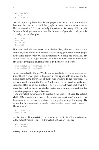
plot(x,y1,'r--')
figure
plot(x,y2,'b-')

Instead of plotting both lines in one graph at the same time, you can also
first plot the sine wave, hold the graph and then plot the second curve.

The command hold is particularly important while using different plot
functions for displaying your data. For instance, if you wish to display the
second graph as a bar plot.

plot(x,y1,'r--')
hold on
bar(x,y2)
hold off
This command plots y1 versus x as dashed line, whereas y2 versus x is
shown as group of blue vertical bars. Alternatively, you can plot both graphs
in the same Figure Window, but in different plots using the subplot. The
syntax subplot(m,n,p) divides the Figure Window into an m-by-n ma-
trix of display regions and makes the p-th display region active.
subplot(2,1,1), plot(x,y1,'r--')
subplot(2,1,2), bar(x,y2)

In our example, the Figure Window is divided into two rows and one col-
umn. The 2D linear plot is displayed in the upper half, whereas the bar
plot appears in the lower half of the Figure Window. In the following, it is
recommended to close the Figure Windows before proceeding to the next
example. After using the function subplot, the following plot would re-
place the graph in the lower display region only, or more general, the last
generated graph in a Figure Window.

An important modification to graphs it the scaling of axis. By default,
MATLAB uses axis limits close to the minima and maxima of the data. Using
the command axis, however, allows to change the settings for scaling. The
syntax for this command is simply axis([xmin xmax ymin ymax]).
The command

plot(x,y1,'r--')
axis([0 pi -1 1])
sets the limits of the x-axis to 0 and ›, whereas the limits of the y-axis are set
to the default values -1 and +1. Important options of axis are

plot(x,y1,'r--')
axis square
making the current axes region square and