Page 55 - MATLAB Recipes for Earth Sciences

46 3 Univariate Statistics

Probability Density Cumulative Distribution
Function Function
1 1
σ=0.5
0.8 0.8

0.6 0.6
f(x) F(x)
0.4 σ=1.0 0.4 σ=1.0
σ=2.0 σ=2.0 σ=0.5
0.2 0.2

0 0
0 2 4 6 0 2 4 6
x x
a b
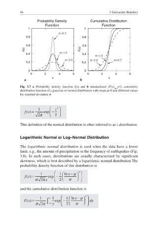
Fig. 3.7 a Probability density function f(x) and b standardized (F(x) =1) cumulative
max
distribution function of a gaussian or normal distribution with mean µ=0 and different values
for standard deviation σ.

This definition of the normal distribution is often referred to as z distribution.

Logarithmic Normal or Log–Normal Distribution

The logarithmic normal distribution is used when the data have a lower
limit, e.g., the amount of precipitation or the frequency of earthquakes (Fig.
3.8). In such cases, distributions are usually characterized by signifi cant
skewness, which is best described by a logarithmic normal distribution The
probability density function of this distribution is

and the cumulative distribution function is