Page 59 - MATLAB Recipes for Earth Sciences

50 3 Univariate Statistics

Probability Density Cumulative Distribution
Function Function
0.5 1
Φ=1 Φ=1
0.4 0.8
Φ=2
0.3 0.6 Φ=2
f(x) Φ=3 F(x) Φ=3
0.2 Φ=4 0.4
Φ=4
0.1 0.2

0 0
0 2 4 6 8 0 2 4 6 8
x x
a b
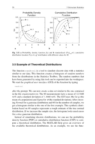
Fig. 3.11 a Probability density function f(x) and b standardized (F(x) =1) cumulative
max
2
distribution function F(x) of a χ distribution with different values for Φ.

3.5 Example of Theoretical Distributions

The function randtool is a tool to simulate discrete data with a statistics
similar to our data. This function creates a histogram of random numbers
from the distributions in the Statistics Toolbox. The random numbers that
have been generated by using this tool can be exported into the workspace.
We start the graphical user interface ( GUI) of the function by typing

randtool
after the prompt. We can now create a data set similar to the one contained
in the fi le organicmatter.txt. The 60 measurements have a mean of 12.3448
wt% and a standard deviation of 1.1660 wt%. The GUI uses Mu for µ (the
mean of a population) and Sigma for σ (the standard deviation). After choos-
ing Normal for a gaussian distribution and 60 for the number of samples, we
get a histogram similar to the one of the first example. This synthetic distri-

bution based on 60 samples represents a rough estimate of the true normal
distribution. If we increase the sample size, the histogram looks much more
like a true gaussian distribution.
Instead of simulating discrete distributions, we can use the probability
density function (PDF) or cumulative distribution function (CDF) to com-
pute a theoretical distribution. The MATLAB Help gives an overview of
the available theoretical distributions. As an example, we use the func-