Page 62 - MATLAB Recipes for Earth Sciences

3.6 The F–Test 53

hypothesized) difference of 0.2.
The second synthetic example shows the performance of the t–test on very
different distributions in the means. The means are 24.3 and 25.5, whereas
the standard deviations are again 1.3 and 1.5, respectively.
clear

load('organicmatter_three.mat');
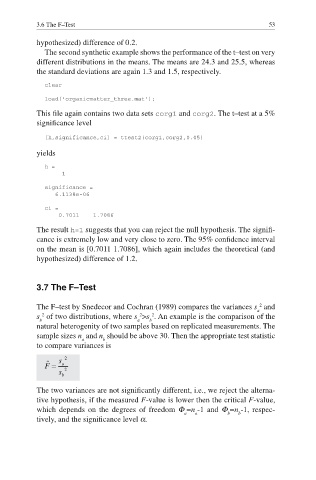
This file again contains two data sets corg1 and corg2. The t–test at a 5%

signifi cance level

[h,significance,ci] = ttest2(corg1,corg2,0.05)
yields
h =
1
significance =
6.1138e-06

ci =
0.7011 1.7086
The result h=1 suggests that you can reject the null hypothesis. The signifi -
cance is extremely low and very close to zero. The 95% confi dence interval
on the mean is [0.7011 1.7086], which again includes the theoretical (and
hypothesized) difference of 1.2.

3.7 The F–Test

The F–test by Snedecor and Cochran (1989) compares the variances s and
2
a
2
2
2
s of two distributions, where s >s . An example is the comparison of the
b a b
natural heterogenity of two samples based on replicated measurements. The
sample sizes n and n should be above 30. Then the appropriate test statistic
a b
to compare variances is

The two variances are not signifi cantly different, i.e., we reject the alterna-
tive hypothesis, if the measured F-value is lower then the critical F-value,
which depends on the degrees of freedom Φ =n -1 and Φ =n -1, respec-
a a b b
tively, and the signifi cance level α.