Page 66 - MATLAB Recipes for Earth Sciences

χ 2
3.8 The –Test 57

corg = load('organicmatter_one.txt');
v = 10 : 0.65 : 14.55;
n_exp = hist(corg,v);

We use this function to create the synthetic frequency distribution n_syn
with a mean of 12.3448 and standard deviation of 1.1660.
n_syn = normpdf(v,12.3448,1.1660);

The data need to be scaled so that they are similar to the original data set.

n_syn = n_syn ./ sum(n_syn);
n_syn = sum(n_exp) * n_syn;
The first line normalizes n_syn to a total of one. The second command scales

n_syn to the sum of n_exp. We can display both histograms for comparison.

subplot(1,2,1), bar(v,n_syn,'r')
subplot(1,2,2), bar(v,n_exp,'b')

Visual inspection of these plots shows that they are similar. However, it
is advisable to use a more quantitative approach. The χ -test explores the
2
squared differences between the observed and expected frequencies. The

Probability Density Function
0.2

2
0.15 Φ=5 χ (Φ=5, α=0.05)
f( ) χ 2 0.1

Donʼt reject Reject null hypothesis!
null hypothesis This decision has a 5%
0.05
without another cause! probability of being wrong.
0
0 2 4 6 8 10 12 14 16 18 20
χ 2
2
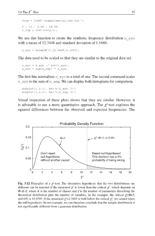
Fig. 3.12 Principles of a χ -test. The alternative hypothesis that the two distributions are
2
2
different can be rejected if the measured χ is lower than the critical χ , which depends on
Φ=K-Z, where K is the number of classes and Z is the number of parameters describing the
theoretical distribution plus the number of variables. In the example, the critical χ (Φ=5,
2
2
2
α=0.05) is 11.0705. If the measured χ =2.1685 is well below the critical χ , we cannot reject
the null hypothesis. In our example, we can therefore conclude that the sample distribution is

not significantly different from a gaussian distribution.