Page 72 - MATLAB Recipes for Earth Sciences

64 4 Bivariate Statistics

where n is the number of xy pairs of data points, s and s the univariate
x y
standard deviations. The numerator of Pearson·s correlation coeffi cient is
known as corrected sum of products of the bivariate data set. Dividing the
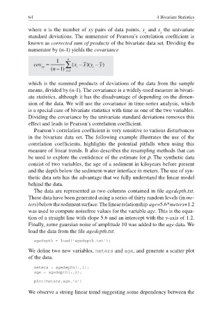
numerator by (n-1) yields the covariance

which is the summed products of deviations of the data from the sample
means, divided by (n-1). The covariance is a widely-used measure in bivari-
ate statistics, although it has the disadvantage of depending on the dimen-
sion of the data. We will use the covariance in time-series analysis, which
is a special case of bivariate statistics with time as one of the two variables.
Dividing the covariance by the univariate standard deviations removes this
effect and leads to Pearson·s correlation coeffi cient.

Pearson·s correlation coefficient is very sensitive to various disturbances
in the bivariate data set. The following example illustrates the use of the

correlation coefficients, highlights the potential pitfalls when using this
measure of linear trends. It also describes the resampling methods that can
be used to explore the confidence of the estimate for ρ. The synthetic data

consist of two variables, the age of a sediment in kiloyears before present
and the depth below the sediment-water interface in meters. The use of syn-
thetic data sets has the advantage that we fully understand the linear model
behind the data.
The data are represented as two columns contained in fi le agedepth.txt.
These data have been generated using a series of thirty random levels (in me-
ters) below the sediment surface. The linear relationship age=5.6*meters+1.2
was used to compute noisefree values for the variable age. This is the equa-
tion of a straight line with slope 5.6 and an intercept with the y-axis of 1.2.
Finally, some gaussian noise of amplitude 10 was added to the age data. We
load the data from the fi le agedepth.txt.

agedepth = load('agedepth.txt');
We defi ne two new variables, meters and age, and generate a scatter plot
of the data.
meters = agedepth(:,1);
age = agedepth(:,2);
plot(meters,age,'o')
We observe a strong linear trend suggesting some dependency between the