Page 75 - MATLAB Recipes for Earth Sciences

4.2 Pearson·s Correlation Coeffi cient 67

rhos1000 = bootstrp(1000,'corrcoef',x,y);

This command first resamples the data a thousand times, calculates the

correlation coefficient for each new subsample and stores the result in the
variable rhos1000. Since corrcoef delivers a 2x2 matrix as mentioned
above, rhos1000 has the dimension 1000x4, i.e., 1000 values for each
element of the 2x2 matrix. Plotting the histogram of the 1000 values of
the second element, i.e., the correlation coeffi cient of (x,y) illustrates the
dispersion of this parameter with respect to the presence or absence of the
outlier. Since the distribution of rhos1000 contains a lot of empty classes,
we use a large number of bins.

hist(rhos1000(:,2),30)
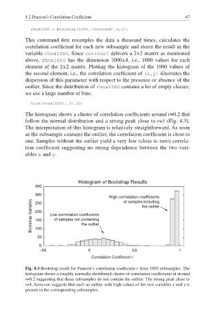
The histogram shows a cluster of correlation coeffi cients around r=0.2 that
follow the normal distribution and a strong peak close to r=1 (Fig. 4.3).
The interpretation of this histogram is relatively straightforward. As soon

as the subsample contains the outlier, the correlation coefficient is close to
one. Samples without the outlier yield a very low (close to zero) correla-
tion coefficient suggesting no strong dependence between the two vari-

ables x and y.

Histogram of Bootstrap Results
350
300
High corrrelation coefficients
Bootstrap Samples 200 Low corrrelation coefficients the outlier
of samples including
250

of samples not containing
150
the outlier
100
50
0
−0.5 0 0.5 1
Correlation Coefficient r

Fig. 4.3 Bootstrap result for Pearson·s correlation coeffi cient r from 1000 subsamples. The
histogram shows a roughly normally-distributed cluster of correlation coefficients at around

r=0.2 suggesting that these subsamples do not contain the outlier. The strong peak close to
r=1, however, suggests that such an outlier with high values of the two variables x and y is
present in the corresponding subsamples.