Page 80 - MATLAB Recipes for Earth Sciences

72 4 Bivariate Statistics

Linear Regression
150
i-th data point
Age of sediments (kyrs) 50 95% Confidence Bounds
95% Confidence Bounds
100

0

−50 Regression line
0 2 4 6 8 10 12 14 16 18 20
Depth in sediment (meters)
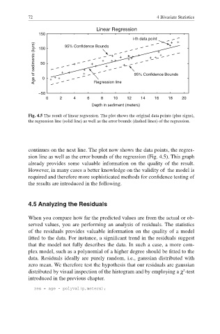
Fig. 4.5 The result of linear regression. The plot shows the original data points (plus signs),
the regression line (solid line) as well as the error bounds (dashed lines) of the regression.

continues on the next line. The plot now shows the data points, the regres-
sion line as well as the error bounds of the regression (Fig. 4.5). This graph
already provides some valuable information on the quality of the result.
However, in many cases a better knowledge on the validity of the model is
required and therefore more sophisticated methods for confidence testing of

the results are introduced in the following.

4.5 Analyzing the Residuals

When you compare how far the predicted values are from the actual or ob-
served values, you are performing an analysis of residuals. The statistics
of the residuals provides valuable information on the quality of a model
fitted to the data. For instance, a significant trend in the residuals suggest

that the model not fully describes the data. In such a case, a more com-
plex model, such as a polynomial of a higher degree should be fi tted to the
data. Residuals ideally are purely random, i.e., gaussian distributed with
zero mean. We therefore test the hypothesis that our residuals are gaussian
2
distributed by visual inspection of the histogram and by employing a χ -test
introduced in the previous chapter.

res = age - polyval(p,meters);