Page 83 - MATLAB Recipes for Earth Sciences

4.6 Bootstrap Estimates of the Regression Coeffi cients 75

1st Regression Coefficient 2st Regression Coefficient
200 200
Slope = 5.6±0.4 150 Y Intercept = 1.3±4.4

Bootstrap Samples 100 Bootstrap Samples 100
150

50
50

0 0
4 5 6 7 −10 0 10 20
Slope Y−Axis Intercept
a b

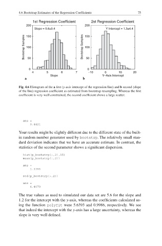
Fig. 4.6 Histogram of the a fi rst (y-axis intercept of the regression line) and b second (slope
of the line) regression coeffi cient as estimated from bootstrap resampling. Whereas the fi rst

coefficient is very-well constrained, the second coefficient shows a large scatter.

ans =
0.4421
Your results might be slightly different due to the different state of the built-
in random number generator used by bootstrp. The relatively small stan-
dard deviation indicates that we have an accurate estimate. In contrast, the
statistics of the second parameter shows a signifi cant dispersion.

hist(p_bootstrp(:,2),15)
mean(p_bootstrp(:,2))

ans =
1.3366
std(p_bootstrp(:,2))

ans =
4.4079

The true values as used to simulated our data set are 5.6 for the slope and
1.2 for the intercept with the y-axis, whereas the coefficients calculated us-

ing the function polyfit were 5.6393 and 0.9986, respectively. We see
that indeed the intercept with the y-axis has a large uncertainty, whereas the
slope is very well defi ned.