Page 88 - MATLAB Recipes for Earth Sciences

80 4 Bivariate Statistics

4.10 Curvilinear Regression

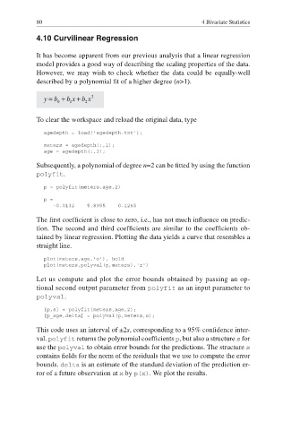
It has become apparent from our previous analysis that a linear regression
model provides a good way of describing the scaling properties of the data.
However, we may wish to check whether the data could be equally-well

described by a polynomial fit of a higher degree (n>1).

To clear the workspace and reload the original data, type
agedepth = load('agedepth.txt');

meters = agedepth(:,1);
age = agedepth(:,2);

Subsequently, a polynomial of degree n=2 can be fitted by using the function

polyfit.
p = polyfit(meters,age,2)
p =
-0.0132 5.8955 0.1265
The fi rst coeffi cient is close to zero, i.e., has not much infl uence on predic-

tion. The second and third coefficients are similar to the coeffi cients ob-
tained by linear regression. Plotting the data yields a curve that resembles a
straight line.

plot(meters,age,'o'), hold
plot(meters,polyval(p,meters),'r')

Let us compute and plot the error bounds obtained by passing an op-
tional second output parameter from polyfit as an input parameter to
polyval.

[p,s] = polyfit(meters,age,2);
[p_age,delta] = polyval(p,meters,s);
This code uses an interval of ±2s, corresponding to a 95% confi dence inter-
val. polyfit returns the polynomial coeffi cients p, but also a structure s for
use the polyval to obtain error bounds for the predictions. The structure s
contains fields for the norm of the residuals that we use to compute the error

bounds. delta is an estimate of the standard deviation of the prediction er-
ror of a future observation at x by p(x). We plot the results.