Page 87 - MATLAB Recipes for Earth Sciences

4.9 Reduced Major Axis Regression 79

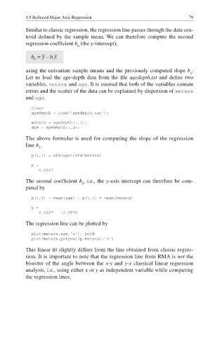
Similar to classic regression, the regression line passes through the data cen-

troid defined by the sample mean. We can therefore compute the second
regression coeffi cient b (the y-intercept),
0

using the univariate sample means and the previously computed slope b .
1
Let us load the age-depth data from the fi le agedepth.txt and defi ne two
variables, meters and age. It is ssumed that both of the variables contain
errors and the scatter of the data can be explained by dispersion of meters
and age.
clear
agedepth = load('agedepth.txt');
meters = agedepth(:,1);
age = agedepth(:,2);

The above formular is used for computing the slope of the regression
line b .
1
p(1,1) = std(age)/std(meters)
p =
6.0367
The second coeffi cient b , i.e., the y-axis intercept can therefore be com-
0
puted by
p(1,2) = mean(age) - p(1,1) * mean(meters)

p =
6.0367 -2.9570

The regression line can be plotted by
plot(meters,age,'o'), hold
plot(meters,polyval(p,meters),'r')

This linear fit slightly differs from the line obtained from classic regres-
sion. It is important to note that the regression line from RMA is not the
bisector of the angle between the x-y and y-x classical linear regression
analysis, i.e., using either x or y as independent variable while computing
the regression lines.