Page 78 - MATLAB Recipes for Earth Sciences

70 4 Bivariate Statistics

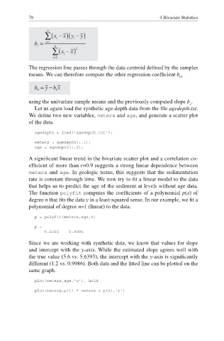
The regression line passes through the data centroid defined by the samples
means. We can therefore compute the other regression coeffi cient b ,
0

using the univariate sample means and the previously computed slope b .
1
Let us again load the synthetic age-depth data from the fi le agedepth.txt.
We defi ne two new variables, meters and age, and generate a scatter plot
of the data.

agedepth = load('agedepth.txt');
meters = agedepth(:,1);
age = agedepth(:,2);

A significant linear trend in the bivariate scatter plot and a correlation co-
efficient of more than r=0.9 suggests a strong linear dependence between

meters and age. In geologic terms, this suggests that the sedimentation
rate is constant through time. We now try to fit a linear model to the data

that helps us to predict the age of the sediment at levels without age data.
The function polyfit computes the coeffi cients of a polynomial p(x) of
degree n that fits the data y in a least-squared sense. In our example, we fi t a

polynomial of degree n=1 (linear) to the data.

p = polyfit(meters,age,1)
p =
5.6393 0.9986

Since we are working with synthetic data, we know that values for slope
and intercept with the y-axis. While the estimated slope agrees well with
the true value (5.6 vs. 5.6393), the intercept with the y-axis is signifi cantly

different (1.2 vs. 0.9986). Both data and the fitted line can be plotted on the
same graph.
plot(meters,age,'o'), hold

plot(meters,p(1) * meters + p(2),'r')