Page 224 - Machine Learning for Subsurface Characterization

194 Machine learning for subsurface characterization

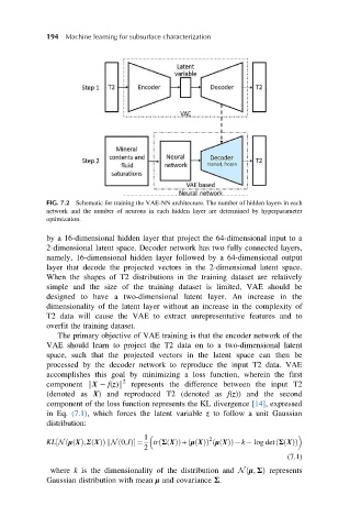
FIG. 7.2 Schematic for training the VAE-NN architecture. The number of hidden layers in each
network and the number of neurons in each hidden layer are determined by hyperparameter
optimization.

by a 16-dimensional hidden layer that project the 64-dimensional input to a
2-dimensional latent space. Decoder network has two fully connected layers,
namely, 16-dimensional hidden layer followed by a 64-dimensional output
layer that decode the projected vectors in the 2-dimensional latent space.
When the shapes of T2 distributions in the training dataset are relatively
simple and the size of the training dataset is limited, VAE should be
designed to have a two-dimensional latent layer. An increase in the
dimensionality of the latent layer without an increase in the complexity of
T2 data will cause the VAE to extract unrepresentative features and to
overfit the training dataset.
The primary objective of VAE training is that the encoder network of the
VAE should learn to project the T2 data on to a two-dimensional latent
space, such that the projected vectors in the latent space can then be
processed by the decoder network to reproduce the input T2 data. VAE
accomplishes this goal by minimizing a loss function, wherein the first
2
component kX f(z)k represents the difference between the input T2
(denoted as X) and reproduced T2 (denoted as f(z)) and the second
component of the loss function represents the KL divergence [14], expressed
in Eq. (7.1), which forces the latent variable z to follow a unit Gaussian
distribution:

1 2
ð
ð
ð
KL Nðμ XðÞ,Σ XðÞÞ kN ð0,Iފ ¼ tr Σ XðÞÞ + μ XðÞÞ μ XðÞð Þ k log det Σ XðÞÞ
½
2
(7.1)
where k is the dimensionality of the distribution and N μ, ΣÞ represents
ð
Gaussian distribution with mean μ and covariance Σ.