Page 226 - Machine Learning for Subsurface Characterization

196 Machine learning for subsurface characterization

and the original T2 distributions. T2 distributions generated by the generator is
fed into the discriminator along with samples taken from the actual, ground-
truth NMR T2 data. The discriminator takes in both real and synthetic T2 and
returns probabilities, a number between 0 and 1, where 1 denotes authenticity
of the T2 and 0 denotes fake/synthetic T2 produced by the generator network.
Generator learns to generate T2 data that get labeled as 1 by the discriminator,
whereas as the discriminator learns to label the T2 data generated by the
generator as 0.
In the first stage of training the GAN-NN, the GAN is trained to synthesize
the NMR T2 similar to those in the training dataset. Generator network G
has two fully connected layers, 6-dimensional input layer followed by two
64-dimensional hidden layers that upscale (transform) the 6-dimensional noise
input to 64-dimensional synthetic NMR T2. Discriminator network D has four
fully connected layers, namely, 64-dimensional input layer, 64-dimensional
and 16-dimensional hidden layers, and finally a 2-dimensional output layer for
classifying each input data fed into the discriminator as either original or
synthetic T2. The primary objective of GAN training is that the generator
network of the GAN should learn to synthesize realistic, physically consistent
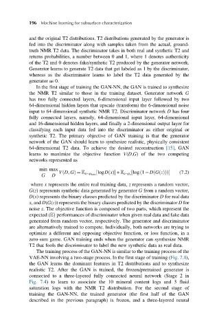
64-dimensional T2 data. To achieve the desired reconstruction [15],GAN
learns to maximize the objective function V(D,G) of the two competing
networks represented as
min max
ð ½ logDxðފ +  z p z ½ log 1 DG zðÞÞފ (7.2)
ð
ð
G D
VD, GÞ ¼  x p data
where x represents the entire real training data, z represents a random vector,
G(z) represents synthetic data generated by generator G from a random vector,
D(x) represents the binary classes predicted by the discriminator D for real data
x, and D(G(z)) represents the binary classes predicted by the discriminator D for
noise z. The objective function is composed of two parts, which represent the
expected (Þ performances of discriminator when given real data and fake data
generated from random vector, respectively. The generator and discriminator
are alternatively trained to compete. Individually, both networks are trying to
optimize a different and opposing objective function, or loss function, in a
zero-sum game. GAN training ends when the generator can synthesize NMR
T2 that fools the discriminator to label the new synthetic data as real data.
The training process of the GAN-NN is similar to the training process of the
VAE-NN involving a two-stage process. In the first stage of training (Fig. 7.4),
the GAN learns the dominant features in T2 distributions and to synthesize
realistic T2. After the GAN is trained, the frozen/pretrained generator is
connected to a three-layered fully connected neural network (Stage 2 in
Fig. 7.4) to learn to associate the 10 mineral content logs and 3 fluid
saturation logs with the NMR T2 distribution. For the second stage of
training the GAN-NN, the trained generator (the first half of the GAN
described in the previous paragraph) is frozen, and a three-layered neural