Page 89 - Machine Learning for Subsurface Characterization

74 Machine learning for subsurface characterization

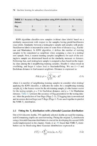
TABLE 3.1 Accuracy of flag generation using KNN classifiers for the testing
dataset.
Flag 2 3 4 5
Accuracy 88% 86% 85% 88%

KNN algorithm classifies new samples (without class labels) based on a
similarity measurment with respect to the samples having predefined/known
class labels. Similarity between a testing/new sample and samples with prede-
fined/known labels is measured in terms of some form of distance (e.g., Euclid-
ean and Manhattan). In KNN algorithm, k defines the number of training
samples to be considered as neighbors when assigning a class to a testing/
new sample. First, k nearest training samples (neighbors) for each of the test-
ing/new sample are determined based on the similarity measure or distance.
Following that, each testing/new sample is assigned a class based on the major-
ity class among the k neighboring training samples. Smaller k values result in
overfitting, and larger k values lead to bias/underfitting. We use k ¼ 5 and
Euclidean distance to find nearest neighbors. Distance is expressed as
v ffiffiffiffiffiffiffiffiffiffiffiffiffiffiffiffiffiffiffiffiffiffiffiffiffi
k
u
p p
u X
D x, y, pð Þ ¼ t ð x n yÞ (3.1)
n¼1
where k is number of neighboring training samples to consider when testing/
applying the KNN classifier, n indicates the index for a neighboring training
sample, x n is the feature vector for the nth training sample, y is the feature vector
for the testing sample, p ¼ 2 for Euclidean distance, and p ¼ 1 for Manhattan
distance. Table 3.1 presents the accuracy of flag generation for the testing data-
set. After the prediction of four flags (Flags 2–5), 22 logging data (conventional
and inversion-derived logs) and 5 flags (Flags 1–5) are used together to predict
the NMR T 2 distribution.

2.5 Fitting the T 2 distribution with a bimodal Gaussian distribution
Out of 416 discrete depths, 354 randomly selected depths are used for training,
and 62 remaining depths are used for testing. Fitting the original T 2 distribution
using a bimodal Gaussian distribution is crucial for developing the second ANN
model implemented in the chapter. Genty et al. [9] found that NMR T 2 distri-
bution can be fitted using three Gaussian distributions expressed as

3
X

fT 0 ¼ A ðÞg i μ , σ i , T 0 (3.2)
2 α i i 2i
i¼1