Page 96 - Machine Learning for Subsurface Characterization

80 Machine learning for subsurface characterization

There are no specific equations or procedures to calculate the number of
neurons (computational units) in each hidden layer. Different combinations
of neurons in each layer were tried for the NMR T 2 prediction. An arithmetic
sequence of the number of neurons in each hidden layer is suggested to generate
high prediction accuracy [12]. Consequently, for the first predictive model that
takes 27 inputs/features and generates 64 outputs/targets, 39 and 51 neurons
were set in the first and second hidden layers of the ANN model, respectively,
because the numbers 27, 39, 51, and 64 approximately form an arithmetic
sequence. This architecture requires 6460 parameters, including the weights
and biases, to be computed/updated during each training step. Following the
same logic, for the second predictive model that has 27 inputs/features and 6
outputs/targets, requires 20 and 13 neurons in the first and second hidden layers
of the ANN model, respectively, such that the sequence 6, 13, 20, and 27 is
nearly an arithmetic sequence. This architecture requires 917 parameters,
including the weights and biases, to be computed/updated during each
training step.
Training functions are the methods to adjust weights and biases to converge
the target functions of ANNs. Target functions quantify errors in learning pro-
cess. ANN learns by minimizing the target functions based on the training func-
tions. Levenberg-Marquardt (LM) backpropagation [13] and conjugate gradient
(CG) backpropagation [14] are two most widely used algorithms for approxi-
mating the training functions, which are the relationships between the features
and targets with the weights and biases of every neuron in the ANN model. LM
backpropagation is suitable for a small number of weights and biases, whereas
CG backpropagation can be applied on large neural networks implementing a
large number of weights and biases. We use CG backpropagation as the training
function for both the ANN-based prediction models. Training time of the ANN
model with LM backpropagation was 10 times more than that with CG back-
propagation. To be specific, scaled conjugate gradient algorithm [14] was used
for our study.
Target function of ANN model adjusts the weights and biases of all neurons
to minimize the errors to ensure the best prediction performance during the
model training. Overfitting is a challenging problem when minimizing the tar-
get function [15]. ANN models cannot learn a generalizable relationship
between targets and features due to overfitting. A simple target function is
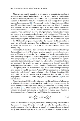
the regularized sum of squared errors (SSE) function expressed as

n P
X 2 X 2
SSE ¼ ð y i ^ y Þ + λ σ (3.10)
i j
i¼1 j¼1
where n is the number of samples/depths in the training/testing dataset and P is
the number of outputs (64 for the first model and 6 for the second model), λ is
penalty parameter, y i is original target at depth i, ^ y is estimated target at depth i,
i
2
and σ j is the variance of predicted target j. Regularization is a popular method to