
Page 253 - Marine Structural Design
P. 253
Chapter I2 A Theory of Nonlinear Finite Element Analysis 229
(12.1)
I
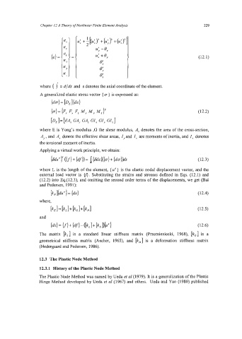
where ( ) = d/ds and s denotes the axial coordinate of the element.
A generalized elastic stress vector { CT } is expressed as:
w = [DE l@4
b>= bX Fy F, Mx My M,)T (12.2)
[DE]= [EAx GAY GA, GZx GZ, GZ,J
where E is Yong’s modulus ,G the shear modulus, A, denotes the area of the cross-section,
A, , and A, denote the effective shear areas, I, and I, are moments of inertia, and I, denotes
the torsional moment of inertia.
Applying a virtual work principle, we obtain:
I..erccrI+ &I)= p4w+ (12.3)
where L is the length of the element, { uc } is the elastic nodal displacement vector, and the
external load vector is v). Substituting the strains and stresses defined in Eqs. (12.1) and
(12.2) into Eq.(12.3), and omitting the second order terms of the displacements, we get (Bai
and Pedersen, 1991):
[kEl(dU‘J= (12.4)
where,
(12.5)
[kE 1 = [kL I+ [k, I+ kD1
and
@I = VI+ k!f> - @L I+ [k, Dbe 1 (12.6)
The matrix [kL] is a standard linear stiffness matrix (Przemieniecki, 1968), [k,] is a
geometrical stiffness matrix (Ancher, 1965), and [kD] is a deformation stiffness matrix
(Nedergaard and Pedersen, 1986).
12.3 The Plastic Node Method
12.3.1 History of the Plastic Node Method
The Plastic Node Method was named by Ueda et a1 (1979). It is a generalization of the Plastic
Hinge Method developed by Ueda et a1 (1967) and others, Ueda and Yao (1980) published