Page 109 - Mathematical Models and Algorithms for Power System Optimization

New Algorithms Related to Power Flow 99

4.6 Formulation of Discrete Optimal Power Flow

4.6.1 Similarities and Differences Between LF and OPF

As explained in Section 4.1.1, the traditional power flow problems of N buses can be expressed
by 2N equations and 4N variables (U, θ, P G , Q G ), and there have to be three types of buses: (1)
PQ bus, P and Q are known (U and θ unknown); (2) PV bus, P and U known (Q and θ unknown,
Q may be Q G or Q L ); and (3) Vθ bus, U and θ are known (P G and Q G unknown). Thus, the
number of variables is equal to the number of equations. However, because variables P and Q
have analytic formulas, U and θ are actually the only variables of power flow, and solving the
power flow finds the distribution situation of voltage and phase angle of the network buses.
Branch power flows P ij and Q ij are functions of U and θ, as well as R and X; thus, P and Q can be
easily calculated by determining U and θ.

If N buses (total 2N variables of U and θ) have 2N added variables (P and Q), the power flow
problems of N buses have 2N equations and 4N variables, so that the number of variables is
greater than the number of equations. Thus, the square power flow equation becomes a
rectangular optimization equation. Such an equation set theoretically has an infinite number of
solutions, among which there are optimized ones depending upon different objectives and how
the variables of the buses are optimized. For the optimization calculation, all buses are
generally treated as PQ buses, so that each bus maintains two equations (P balance equation and
Q balance equation), and the number of equations is 2N. If the 2N equations and 4N variables
are used to solve the traditional power flow, just set the upper and lower limits of P and Q of the
PQ bus as the known P and Q values, the upper and lower limits of P and U of the PV bus as the
known P and U values, and the upper and lower limits of U and θ of the Vθ bus (balance bus) as
the known U and θ values. P and Q may be deemed as P G and Q G or P L and Q L . The load
optimization and reactive power optimization are discussed in Chapters 5 and 6, respectively.

Therefore, traditional power flow calculation is equivalent so that two of the four variables for
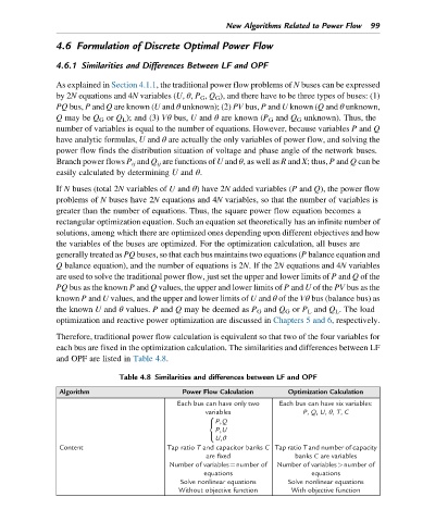
each bus are fixed in the optimization calculation. The similarities and differences between LF
and OPF are listed in Table 4.8.

Table 4.8 Similarities and differences between LF and OPF
Algorithm Power Flow Calculation Optimization Calculation

Each bus can have only two Each bus can have six variables:
P, Q, U, θ, T, C
variables
8
P,Q
<
P,U
U,θ
:
Content Tap ratio T and capacitor banks C Tap ratio T and number of capacity
are fixed banks C are variables
Number of variables¼number of Number of variables>number of
equations equations
Solve nonlinear equations Solve nonlinear equations
Without objective function With objective function