Page 116 - Mathematical Models and Algorithms for Power System Optimization

106 Chapter 4

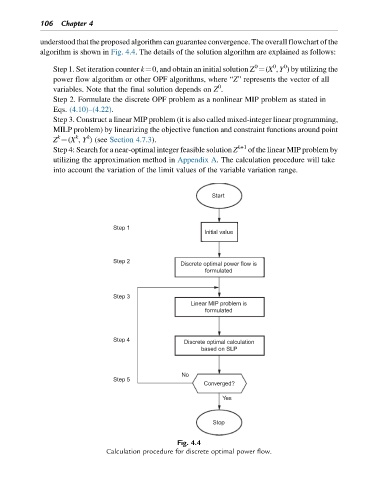
understood that the proposed algorithm can guarantee convergence. The overall flowchart of the
algorithm is shown in Fig. 4.4. The details of the solution algorithm are explained as follows:

0 0 0
Step 1. Set iteration counter k¼0, and obtain an initial solution Z ¼(X , Y ) by utilizing the
power flow algorithm or other OPF algorithms, where “Z” represents the vector of all
0
variables. Note that the final solution depends on Z .
Step 2. Formulate the discrete OPF problem as a nonlinear MIP problem as stated in
Eqs. (4.10)–(4.22).
Step 3. Construct a linear MIP problem (it is also called mixed-integer linear programming,
MILP problem) by linearizing the objective function and constraint functions around point
k
k
k
Z ¼(X , Y ) (see Section 4.7.3).
Step 4: Search for a near-optimal integer feasible solution Z k+1 of the linear MIP problem by
utilizing the approximation method in Appendix A. The calculation procedure will take
into account the variation of the limit values of the variable variation range.

Start

Step 1
Initial value

Step 2 Discrete optimal power flow is
formulated

Step 3
Linear MIP problem is
formulated

Step 4
Discrete optimal calculation
based on SLP

No
Step 5
Converged?
Yes

Stop

Fig. 4.4
Calculation procedure for discrete optimal power flow.