Page 118 - Mathematical Models and Algorithms for Power System Optimization

108 Chapter 4

during the iterative solving process for the mixed-integer LP problem, the limits of the
variables shall be adjusted to solve the nonlinear OPF problem. The calculation process is
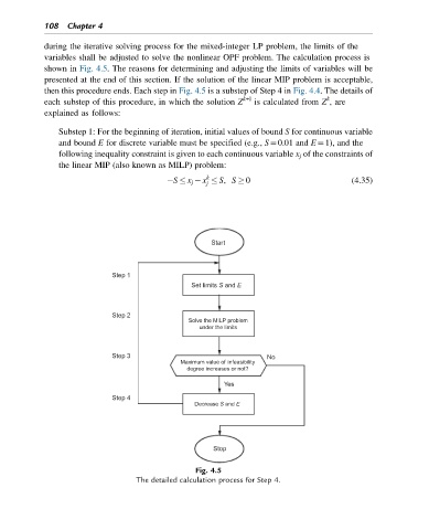
shown in Fig. 4.5. The reasons for determining and adjusting the limits of variables will be
presented at the end of this section. If the solution of the linear MIP problem is acceptable,
then this procedure ends. Each step in Fig. 4.5 is a substep of Step 4 in Fig. 4.4. The details of
k+l k
each substep of this procedure, in which the solution Z is calculated from Z , are
explained as follows:

Substep 1: For the beginning of iteration, initial values of bound S for continuous variable
and bound E for discrete variable must be specified (e.g., S¼0.01 and E¼1), and the
following inequality constraint is given to each continuous variable x j of the constraints of
the linear MIP (also known as MILP) problem:

k
S x j x S, S 0 (4.35)
j

Start

Step 1
Set limits S and E

Step 2
Solve the MILP problem
under the limits

Step 3 No
Maximum value of infeasibility
degree increases or not?
Yes
Step 4
Decrease S and E

Stop

Fig. 4.5

The detailed calculation process for Step 4.