Page 172 - Mathematical Models and Algorithms for Power System Optimization

Discrete Optimization for Reactive Power Planning 163

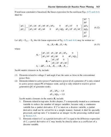
If nonlinear constraint is linearized, the linear expression for the nonlinear Eqs. (6.5) and (6.6)
shall be:

ΔU
2 3
Δθ
6 7
6 7
6 7
ΔF 1 ∂F 1 =∂U ∂F 1 =∂θ ∂F 1 =∂P G 0 ∂F 1 =∂T 0 6 ΔP G 7
¼ 6 7 (6.12)
ΔF 2 ∂F 2 =∂U ∂F 2 =∂θ 0 ∂F 2 =∂Q G ∂F 2 =∂T ∂T 2 =∂C 6 7
6 ΔQ G 7
6 7
ΔT 5
4
ΔG
Let ΔX k ¼X k+1 X k ; the kth linear expression of Eq. (6.5) and (6.6) may be written as:
(6.13)
A k 1 X k + B k 1 Y k ¼ b k
where

∂F 1 =∂U ∂F 1 =∂θ ∂F 1 =∂P G 0
A k ¼
∂F 2 =∂U ∂F 2 =∂θ 0 ∂F 2 =∂Q G
∂F 1 =∂T 0

B k ¼
∂F 2 =∂T ∂F 2 =∂C
b k ¼ ΔF k 1 + A k 1 X k 1 + B k 1 Y k 1
Jacobi matrix elements in A k include:

(1) Elements related to voltage U and angle θ are the same as those in the conventional
power flow.
(2) Elements related to active power P and reactive power Q of a generator (P is only related
to active power output PS of balance node, and Q is only related to reactive power
generation QG of generator node).

∂F 1i =∂P Si ¼ 1:0
∂F 2i =∂Q Gi ¼ 1:0
Jacobi matrix elements in the matrix B k include:
1. Elements related to tap ratio: In this chapter, T is temporarily treated as a continuous
variable to reduce the number of integer variables, because only a continuous
variable has a partial derivative. If T is taken as a discrete variable, a partial
derivative shall not be solved for in a simple manner. Instead, it shall be specially
processed, and tap ratio T is treated as an integer via the processing method used
in Section 6.5.
2. Elements related to C: as a partial derivative of C is equal to the difference expression
of C, a partial derivative of C may hereby be directly taken as a coefficient of a
discrete variable.