Page 180 - Mathematical Models and Algorithms for Power System Optimization

Discrete Optimization for Reactive Power Planning 171

be processed can be as many as 69. The overall results of Cases 1–5 show that the algorithm can
effectively deal with integer variables and solve the reactive power optimizations of real-scale
system within 1min.

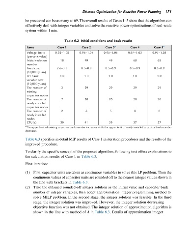
Table 6.2 Initial conditions and basic results
Items Case 1 Case 2 Case 3 a Case 4 Case 5 a

Voltage limits 0.92–1.08 0.95–1.05 0.95–1.05 0.97–1.03 0.97–1.03
(per-unit value)
Initial violation 18 49 49 68 68
number
Fixed cost 2.6–3.8 0.5–0.9 0.5–0.9 0.5–0.9 0.5–0.9
(10,000 yuan)
Per bank 1.0 1.0 1.0 1.0 1.0
variable cost
(10,000 yuan)
The number of 3 29 29 29 29
existing
capacitor nodes
The number of 7 20 20 20 20
newly installed
capacitor nodes
The number of 2 6 5 8 8
newly installed
nodes
CPU(s) 39 41 39 37 57
a
The upper limit of existing capacitor bank number increases while the upper limit of newly installed capacitor bank number
decreases.
Table 6.3 specifies in detail MIP results of Case 1 in iteration procedures and the results of the
improved procedure.

To clarify the specific concept of the proposed algorithm, following text offers explanations to
the calculation results of Case 1 in Table 6.3.
First iteration:

(1) First, capacitor units are taken as continuous variables to solve this LP problem. Then the
continuous values of capacitor units are rounded off to the nearest integer values shown in
the line with brackets in Table 6.3.
(2) Take the obtained rounded-off integer solution as the initial value and capacitor bank
number of integer variables, then adopt approximation integer programming method to
solve MILP problem. In the second stage, the integer solution was feasible. In the third
stage, the integer solution was improved. However, the integer solution decreasing
objective function was not obtained. The integer solution of approximation algorithm is
shown in the line with method of A in Table 6.3. Details of approximation integer