Page 238 - Mathematical Models and Algorithms for Power System Optimization

230 Chapter 7

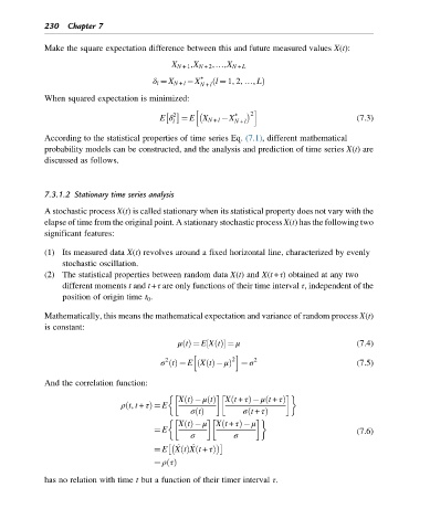
Make the square expectation difference between this and future measured values X(t):

X N +1 ,X N +2 ,…,X N + L
∗
δ l ¼ X N + l X ð l ¼ 1, 2, …, LÞ
N + l
When squared expectation is minimized:
h i
∗ 2
2
E δ ¼ EX N + l X (7.3)
l N + l
According to the statistical properties of time series Eq. (7.1), different mathematical
probability models can be constructed, and the analysis and prediction of time series X(t) are
discussed as follows.

7.3.1.2 Stationary time series analysis

A stochastic process X(t) is called stationary when its statistical property does not vary with the
elapse of time from the original point. A stationary stochastic process X(t) has the following two
significant features:

(1) Its measured data X(t) revolves around a fixed horizontal line, characterized by evenly
stochastic oscillation.
(2) The statistical properties between random data X(t) and X(t+τ) obtained at any two
different moments t and t+τ are only functions of their time interval τ, independent of the
position of origin time t 0 .

Mathematically, this means the mathematical expectation and variance of random process X(t)
is constant:
μ tðÞ ¼ EX tðފ ¼ μ (7.4)
½
h i
2 2 2
σ tðÞ ¼ EX tðÞ μð Þ ¼ σ (7.5)
And the correlation function:

XtðÞ μ tðÞ Xt + τÞ μ t + τÞ
ð
ð
ρ t, t + τÞ ¼ E
ð
σ tðÞ σ t + τÞ
ð
XtðÞ μ Xt + τÞ μ

ð
¼ E (7.6)
σ σ
^ ^

¼ E XtðÞXt + τÞ
ð
¼ ρτðÞ
has no relation with time t but a function of their timer interval τ.