Page 239 - Mathematical Models and Algorithms for Power System Optimization

Optimization Method for Load Frequency Feed Forward Control 231

7.3.1.3 Nonstationary time series analysis
The so-called nonstationary time series refer to a very wide range of physical data with their
statistical properties varying with time. Most of physical data encountered in the practical
problem are generally nonstationary. A group of original measured data are assumed to be
stationary only when the primal problems are simplified or roughly approximated. The
nonstationary time series are so complicated that there is no generalized method to deal with it.
The high-order difference method, namely the difference method, may be used to stabilize
it shown as follows:
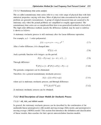
A stationary stochastic process is still stationary after the linear difference operation.

For example, a d 1 order polynomial:

ftðÞ ¼ c 0 + c 1 t + ⋯ + c d 1 t d 1 (7.7)
After d order difference, it is changed into:

d
r ftðÞ ¼ 0 (7.8)
And a periodic function with integer s as the period:
ð
ð
PtðÞ ¼ Pt + nsÞ n ¼ 1, 2, …Þ (7.9)
Through difference
s
ð
r s PtðÞ ¼ 1 Bð ÞPtðÞ ¼ PtðÞ Pt sÞ (7.10)
The periodic component can be eliminated.

Therefore, for a general nonstationary stochastic process:

XtðÞ ¼ ftðÞ + PtðÞ + η tðÞ (7.11)
where η(t) is stationary stochastic process, and through difference:
d d
r r s XtðÞr r s η tðÞ (7.12)
A stationary stochastic process can be obtained.

7.3.2 Brief Descriptions of Linear Models for Stochastic Process

7.3.2.1 AR, MA, and ARMA models

In general, the stationary stochastic process can be described by the combination of the
multiorder linear autoregressive (AR) model, moving average (MA) model, and autoregressive
moving average (ARMA) model. This section first introduces the definition and classification
of linear models, then searches for their special autocorrelation function models.