Page 243 - Mathematical Models and Algorithms for Power System Optimization

Optimization Method for Load Frequency Feed Forward Control 235

To make S minimal, when k p, it shall take:
ϕ ð 1 j pÞ

ϕ ¼ j (7.29)
kj
0 ð p +1 j k, k ¼ p, p +1⋯Þ
In particular, when k¼p+1, …:
ϕ ¼ 0
kk
It can be seen that the partial autocorrelation function of AR process is truncated; truncation of
ϕ kk is the unique characteristic of AR process.
For MA and ARMA processes, the partial autocorrelation function is still defined by Eq. (7.27),
however, ϕ kk is not truncated but tailing. The autocorrelation function and partial
autocorrelation function of ARMA process are not derived here; only their results as shown in
Table 7.1.

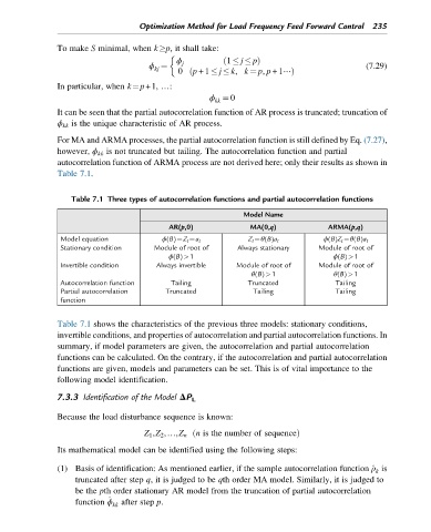
Table 7.1 Three types of autocorrelation functions and partial autocorrelation functions
Model Name
AR(p,0) MA(0,q) ARMA(p,q)
ϕ(B)¼Z t ¼a t Z t ¼θ(B)a t ϕ(B)Z t ¼θ(B)a t
Model equation
Stationary condition Module of root of Always stationary Module of root of
ϕ(B)>1 ϕ(B)>1
Invertible condition Always invertible Module of root of Module of root of
θ(B)>1 θ(B)>1
Autocorrelation function Tailing Truncated Tailing
Partial autocorrelation Truncated Tailing Tailing
function

Table 7.1 shows the characteristics of the previous three models: stationary conditions,
invertible conditions, and properties of autocorrelation and partial autocorrelation functions. In
summary, if model parameters are given, the autocorrelation and partial autocorrelation
functions can be calculated. On the contrary, if the autocorrelation and partial autocorrelation
functions are given, models and parameters can be set. This is of vital importance to the
following model identification.

7.3.3 Identification of the Model ΔP L

Because the load disturbance sequence is known:

Z 1 ,Z 2 ,…,Z n ð n is the number of sequenceÞ
Its mathematical model can be identified using the following steps:

(1) Basis of identification: As mentioned earlier, if the sample autocorrelation function ^ ρ is
k
truncated after step q, it is judged to be qth order MA model. Similarly, it is judged to
be the pth order stationary AR model from the truncation of partial autocorrelation
^
function ϕ after step p.
kk