Page 98 - Mathematical Models and Algorithms for Power System Optimization

88 Chapter 4

In SA, the temperature of the system is slowly lowered to 0°C; if the temperature falls slowly
enough, the system should end up within the minimum energy states of sufficiently low energy.
Hence SA algorithm can be viewed as minimizing the cost function (energy) over a finite set of
the system state. By simulating such an annealing process, global minimum cost solutions can
be found for very large optimization problems.

4.2.3 Way of Modifying Iteration Step Size by SA Method

Mathematically, this is a problem of solving a set of multivariate nonlinear equations. The basic
principles of the previously discussed algorithms all depend on iterative processes. In these
algorithms, the modified size of each iterative step is calculated from the iterative process in the
previous step. The iterative process approaching to final solution is generally monotonous. In
other words, when the iterative process is in a form of monotonous descending downhill, the
solution is convergent. When it is in a form of monotonous ascending uphill or zigzags, a
convergent solution is difficult to obtain.

4.2.4 Way of Constructing a Nonlinear Quadratic Objective Function

To apply the SA technique to solve the power flow problem in power systems, the modified bus
powerequationinthepowerflowcalculationmaybeusedtoconstructaquadraticfunctionthatis
analogous to the nonlinear objective function. The specific mathematical model is as follows:
n o
X X
2
min FXðÞ ¼ ΔP + ΔQ 2
i i
4.3 Formulation of Unconstrained Power Flow Model with Nonlinear
Quadratic Objective Function

4.3.1 Notation

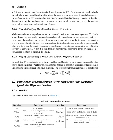
The mathematical notations are listed in Table 4.1.

Table 4.1 Mathematical notations
Notation Description Notation Description

N Set of all buses P iL ,Q iL Active and reactive load at bus i
Vector of voltage magnititude value and
X=(U,θ) P iLO ,Q iLO Initial active and reactive load at bus i
phase angle
Active and reactive power injected at Characterization factor of static voltage
P i ,Q i
bus i a P ,b P ,c P under active load
Active and reactive power flow from bus i Characterization factor of static voltage
P ij ,Q ij
to bus j a Q ,b Q ,c Q under reactive load
Active and reactive generated power at
P iG ,Q iG
bus i