Page 100 - Mathematical Models and Algorithms for Power System Optimization

90 Chapter 4

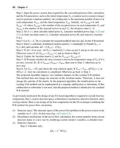
Step 1: Input the power system data required by the conventional power flow calculation
and the SA parameters, such as the initial temperature T 0 , a random seed (a nonzero integer
used to generate a random number), the cooling ratio b, the maximum number of moves at
each temperature N max , and the final temperature T min . Initially, set N accept ¼0, and
N reject ¼0; where N accept is the number of the accepted moves in each temperature T k , and
N reject is the number of the rejected moves in each T k . Set iteration count k¼0.
Step 2: Set k¼1, then calculate initial point X k . Linearize modified power Eqs. (4.2) and
(4.3) to form Jacobian matrix J k . Calculate mismatch power M k and objective function
F(X k ).
1
Step 3: Use X k ¼J k M k to calculate the original modified step size ΔX k for the N-R method.
Step 4: Select a uniformly distributed random number r¼random[0,1]. Perturb X k+1 ¼
X k +rΔX k and calculate ΔF¼F(X k+1 ) F(X k ).
Step 5: If ΔF<0 or exp( ΔF/T k )>random[0,1], then accept X and go to the next step.
Otherwise reject X, let N reject ¼N reject +1, and go back to Step 4.
Step 6: Update the Jacobian matrix J k and let N accept ¼N accept +1.
Step 7: ① Evaluate whether the stop criterion is met in the temperature range of T k ;ifitis
not met, execute ②; ② if N accept +N reject <N max , then turn to Step 3; otherwise go to
next step.
Step 8: Let T k+1 ¼bT k and check the stop criterion again. If T k+1 <T min , ΔF(X k )<ε,or
0
M(X k )<ε , then the calculation is completed. Otherwise go back to Step 3.
The proposed algorithm imposes very minimal changes on the existing N-R method.
This method does not change the structure of the Jacobian matrix. Therefore, it does not
change the sparsity of the matrix. In the proposed algorithm, the modifications to the
existing N-R method can be implemented in a separate subfunction or subroutine. If this
subfunction or subroutine is not used, then the proposed method is identical to the standard
N-R method.

As previously mentioned, the design of any SA-based algorithm is required to include four key
components, that is, system structure space, a disturbance mechanism, objective function, and a
cooling scheme. Here is our design of the four components for the SA technique combining the
N-R method for power flow calculation.

(1) Structure space: The structure space of the power flow problem in the power system is the
variable set X¼X(U, θ) that meet Eqs. (4.2) and (4.3).
(2) Disturbance mechanism: In the power flow calculation, the system transfers from current
structure status to a new one by modifying current iterative variables, as detailed here:
(3) Objective function:
Step 1: Calculate ΔX k :

1
ðÞ
ΔX k ¼ J MX k