Page 185 - Mathematical Techniques of Fractional Order Systems

Fractional Order Error Models With Parameter Constraints Chapter | 6 173

" # " #
2
2
Ð t Oe 1 ðτÞO dτ Ð t Oe 2 ðτÞO dτ
α2ε t 0 α2ε t 0
lim t 5 lim t
t-N t t-N t
" Ð t OξðτÞO dτ #
2
α2ε t 0
5 lim t 5 0 ð6:35Þ
t-N t
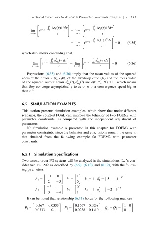
which also allows concluding that
" # " #
2
2
Ð t e ðτÞdτ Ð t e ðτÞdτ
α2ε t 0 m 1 α2ε t 0 m 2
lim t 5 lim t 5 0 ð6:36Þ
t-N t t-N t
Expressions (6.35) and (6.36) imply that the mean values of the squared
norm of the errors e 1 ðtÞ; e 2 ðtÞ, of the auxiliary error ξðtÞ and the mean value
2
2
of the squared output errors e ðtÞ; e ðtÞ are oðt ε2α Þ, ’ε . 0, which means
m 1 m 2
that they converge asymptotically to zero, with a convergence speed higher
than t 2α .
6.5 SIMULATION EXAMPLES
This section presents simulation examples, which show that under different
scenarios, the coupled FOAL can improve the behavior of two FOEM2 with
parameter constraints, as compared with the independent adjustment of
parameters.
No simulation example is presented in this chapter for FOEM3 with
parameter constraints, since the behavior and conclusions remain the same to
that obtained from the following example for FOEM2 with parameter
constraints.

6.5.1 Simulation Specifications
Two second order FO systems will be analyzed in the simulations. Let’s con-
sider two FOEM2 as described by (6.9), (6.10), and (6.12), with the follow-
ing parameters.
21 0 1 T

A 1 5 b 1 5 k 1 5 1 θ 5 5 21
1
2 25 0

23 1 0 T
A 2 5 b 2 5 k 2 5 1 θ 5223
2
0 24 1
It can be noted that relationship (6.11) holds for the following matrices

0:567 0:0333 0:1667 0:0238 1 0
P 1 5 P 2 5 Q 1 5 Q 2 5
0:0333 0:1 0:0238 0:1310 0 1