Page 407 - Mathematical Techniques of Fractional Order Systems

396 Mathematical Techniques of Fractional Order Systems

(A) (B) ρ ρ ρ ρ
50 ρ ρ ρ ρ 50
max ρ ρ ρ ρ ρ ρ ρ ρ max
b+ b+
0 0

ρ ρ ρ ρ ρ ρ ρ ρ ρ ρ ρ ρ
–50 min b– –50 b– ρ ρρ ρ
min
0.5 1 1.5 2 0.5 1 1.5 2
a α α α α
4
(C) (D) X
10 X max+ X max+
X max–
max– 2 X
5 X min– min–
0 0

0 0.5 1 1.5 2 0 1 2 3
a
b
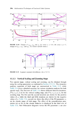
FIGURE 13.14 Changes of ρ max , ρ min and ρ (A) versus a, α 5 0:5, (B) versus α; a 5 3,
b
changes of x max1 , x max2 and x min2 (C) versus b and (D) versus a.

0

MLE –5

α α α α = 0.3
α α α α = 0.7
–10
0 1 2 3
ρ ρ ρ ρ
FIGURE 13.15 Lyapunov exponent with different α for a 5 b 5 2.

13.3.3 Vertical Scaling and Zooming Maps

Two special maps, vertical scaling and zooming, can be obtained through
using the scaling parameters as explained in Section 13.2.2.1. The dynamics
analyses equations of both maps are summarized in Table 13.5, while
Table 13.6 gives a detailed summary for various simulation analyses for both
special maps. The first row of Table 13.6 shows different function iterations,
m
m
f ðx; r; ρ; α; 1; bÞ for the vertical scaling map, and f ðx; r; ρ; α; a; 1Þ, for the
zooming map. The first and the second iterations are shown for the positive
values of ρ, while the third and fifth iterations are shown for the negative
values of ρ. Table 13.6, second row shows the effect of the FO parameter α,
on the chaotic range of both maps. The effect of the generalization para-
meters ðaÞ or ðbÞ on the chaotic behavior is displayed in the third row of
Table 13.6. New bifurcation diagrams versus the FO parameter α are also