Page 403 - Mathematical Techniques of Fractional Order Systems

392 Mathematical Techniques of Fractional Order Systems

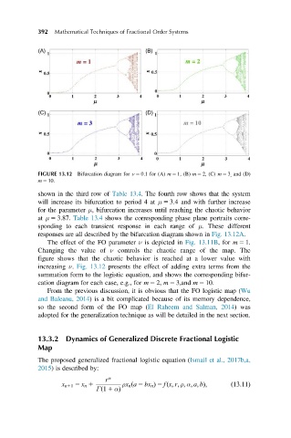
FIGURE 13.12 Bifurcation diagram for ν 5 0:1 for (A) m 5 1, (B) m 5 2, (C) m 5 3 , and (D)
m 5 10.
shown in the third row of Table 13.4. The fourth row shows that the system
will increase its bifurcation to period 4 at μ 5 3:4 and with further increase
for the parameter μ, bifurcation increases until reaching the chaotic behavior
at μ 5 3:87. Table 13.4 shows the corresponding phase plane portraits corre-
sponding to each transient response in each range of μ. These different
responses are all described by the bifurcation diagram shown in Fig. 13.12A.
The effect of the FO parameter ν is depicted in Fig. 13.11B, for m 5 1.
Changing the value of ν controls the chaotic range of the map. The
figure shows that the chaotic behavior is reached at a lower value with
increasing ν. Fig. 13.12 presents the effect of adding extra terms from the
summation form to the logistic equation, and shows the corresponding bifur-
cation diagram for each case, e.g., for m 5 2, m 5 3,and m 5 10.
From the previous discussion, it is obvious that the FO logistic map (Wu
and Baleanu, 2014) is a bit complicated because of its memory dependence,
so the second form of the FO map (El Raheem and Salman, 2014)was
adopted for the generalization technique as will be detailed in the next section.

13.3.2 Dynamics of Generalized Discrete Fractional Logistic
Map
The proposed generalized fractional logistic equation (Ismail et al., 2017b,a,
2015) is described by:
r α
x n11 5 x n 1 ρx n ða 2 bx n Þ 5 fðx; r; ρ; α; a; bÞ; ð13:11Þ
Γð1 1 αÞ