
Page 401 - Mathematical Techniques of Fractional Order Systems
P. 401
390 Mathematical Techniques of Fractional Order Systems
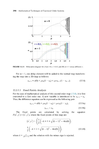
FIGURE 13.11 Bifurcation diagram for (A)m 5 0, ν 5 0:5, and (B) m 5 1 versus different ν.
For m 5 1, one delay element will be added to the normal map transform-
ing the map into a 2D-map as follows:
x n11 5 xð0Þ 1 μx n ð1 2 x n Þ 1 μνx n21 ð1 2 x n21 Þ: ð13:8Þ
13.3.1.1 Fixed Points Analysis
For the ease of mathematical analysis of this second order map (13.8),itis first
converted to a first order one. A new variable is introduced to be y n11 5 x n .
Thus, the difference equation can be expressed as the following pair:
x n11 5 xð0Þ 1 μx n ð1 2 x n Þ 1 μνy n ð1 2 y n Þ; ð13:9aÞ
y n11 5 x n : ð13:9bÞ
The fixed points are calculated by solving the equation
Fðx ; y Þ 5 ðx ; y Þ, where the fixed points of this map are:
q ffiffiffiffiffiffiffiffiffiffiffiffiffiffiffiffiffiffiffiffiffiffiffiffiffiffiffiffiffiffiffiffiffiffi
1
2
x ; y 5 k 1 1 1 ðk 1Þ 4kxð0Þ ;
2
!
q ffiffiffiffiffiffiffiffiffiffiffiffiffiffiffiffiffiffiffiffiffiffiffiffiffiffiffiffiffiffiffiffiffiffi
1 2
k 1 1 1 ðk 1Þ 4kxð0Þ ; ð13:10Þ
2
where k 5 1 and the solution with the minus sign is rejected.
μð1 1 νÞ