Page 172 - Matrices theory and applications

9.4. The Tridiagonal Case
This proof gives a slightly more precise result than what was claimed: By
−1
Nx A on the unit ball, which is compact,
taking the supremum of M
we obtain M
The main application of this lemma is the following theorem.
Theorem 9.3.1 If A is Hermitian positive definite, then the relaxation
method converges if and only if |ω − 1| < 1.
Proof −1 N < 1 for the matrix norm induced by · A. 155
We have seen in Proposition 9.2.1 that the convergence implies |ω − 1| <
1. Let us see the converse. We have E = F and D = D.Thus
∗
∗
2
1 1 1 −|ω − 1|
∗
M + N = + − 1 D = D.
ω ¯ ω |ω| 2
Since D is positive definite, M + N is positive definite if and only if
∗
|ω − 1| < 1.
However, Lemma 9.3.1 does not apply to the Jacobi method, since the
∗
hypothesis (A positive definite) does not imply that M + N = D + E + F
must be positive definite. We shall see in an exercise that this method
diverges for certain matrices A ∈ HPD n , though it converges when A ∈
HPD n is tridiagonal.
9.4 The Tridiagonal Case
We consider here the case of tridiagonal matrices A, frequently encountered
in the approximation of partial differential equations by finite differences
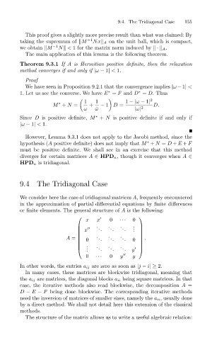
or finite elements. The general structure of A is the following:
 
x x 0 ··· 0
. . .
 . . . . 
x . . . . . 

 
. . .
 . . .  .

0 . . . 0
A = 

 . . . . 
 . . . . . . . . y 

0 ··· 0 y y
In other words, the entries a ij are zero as soon as |j − i|≥ 2.
In many cases, these matrices are blockwise tridiagonal, meaning that
the a ij are matrices, the diagonal blocks a ii being square matrices. In that
case, the iterative methods also read blockwise, the decomposition A =
D − E − F being done blockwise. The corresponding iterative methods
need the inversion of matrices of smaller sizes, namely the a ii , usually done
by a direct method. We shall not detail here this extension of the classical
methods.
The structure of the matrix allows us to write a useful algebraic relation: