Page 176 - Matrices theory and applications

ρ(L ω)

ω J − 1 1 9.5. The Method of the Conjugate Gradient 159
ω
1 ω J 2

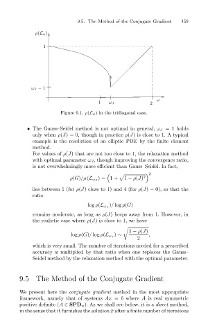
Figure 9.1. ρ(L ω) in the tridiagonal case.

• The Gauss–Seidel method is not optimal in general; ω J =1 holds
only when ρ(J) = 0, though in practice ρ(J) is close to 1. A typical
example is the resolution of an elliptic PDE by the finite element
method.
For values of ρ(J) that are not too close to 1, the relaxation method
with optimal parameter ω J , though improving the convergence ratio,
is not overwhelmingly more efficient than Gauss–Seidel. In fact,
2

)= 1+ 1 − ρ(J) 2
ρ(G)/ρ (L ω J
lies between 1 (for ρ(J) close to 1) and 4 (for ρ(J) = 0), so that the
ratio
)/ log ρ(G)
log ρ(L ω J
remains moderate, as long as ρ(J) keeps away from 1. However, in
the realistic case where ρ(J)is close to 1, we have
%
1 − ρ(J)
) ∼ ,
log ρ(G)/ log ρ(L ω J
2
which is very small. The number of iterations needed for a prescribed
accuracy is multiplied by that ratio when one replaces the Gauss–
Seidel method by the relaxation method with the optimal parameter.

9.5 The Method of the Conjugate Gradient

We present here the conjugate gradient method in the most appropriate
framework, namely that of systems Ax = b where A is real symmetric
positive definite (A ∈ SPD n ). As we shall see below, it is a direct method,
in the sense that it furnishes the solution ¯x after a finite number of iterations