Page 115 - Matrix Analysis & Applied Linear Algebra

3.6 Properties of Matrix Multiplication 109

7.3.5, a more sophisticated approach is discussed, but for now we will use the
“brute force” method of successively powering P until a pattern emerges. The
first several powers of P are shown below with three significant digits displayed.

.375 .625 .344 .656 .328 .672
P 2 = P 3 = P 4 =
.312 .687 .328 .672 .332 .668

.334 .666 .333 .667 .333 .667
P 5 = P 6 = P 7 =
.333 .667 .333 .667 .333 .667
This sequence appears to be converging to a limiting matrix of the form

1/32/3
k
P ∞ = lim P = ,
k→∞ 1/32/3
so the limiting population distribution is

1/32/3
T
k
k
T
T
T
p = lim p = lim p T = p lim T =( n 0 s 0 )
∞ k 0 0 1/32/3
k→∞ k→∞ k→∞

n 0 + s 0 2(n 0 + s 0 )
= =( 1/32/3) .
3 3
Therefore, if the migration pattern continues to hold, then the population dis-
tribution will eventually stabilize with 1/3 of the population being in the North
and 2/3 of the population in the South. And this is independent of the initial
distribution! The powers of P indicate that the population distribution will be
practically stable in no more than 6 years—individuals may continue to move,
but the proportions in each region are essentially constant by the sixth year.
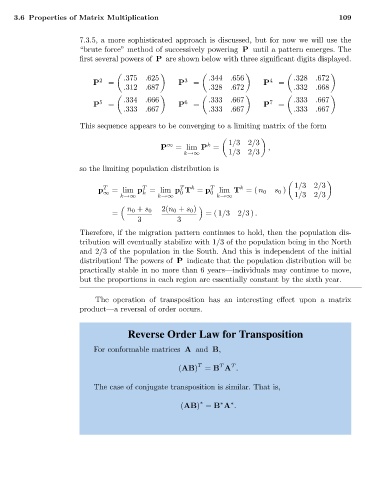
The operation of transposition has an interesting effect upon a matrix
product—a reversal of order occurs.
Reverse Order Law for Transposition
For conformable matrices A and B,

T
T
T
(AB) = B A .
The case of conjugate transposition is similar. That is,
∗
(AB) = B A .
∗
∗