Page 118 - Matrix Analysis & Applied Linear Algebra

112 Chapter 3 Matrix Algebra
Example 3.6.7

Reducibility. Suppose that T n×n x = b represents a system of linear equa-
tions in which the coefficient matrix is block triangular. That is, T can be
partitioned as

A B
T = , where A is r × r and C is n − r × n − r. (3.6.3)
0 C

If x and b are similarly partitioned as x = x 1 and b = b 1 , then block
x 2 b 2
multiplication shows that Tx = b reduces to two smaller systems

Ax 1 + Bx 2 = b 1 ,
Cx 2 = b 2 ,

so if all systems are consistent, a block version of back substitution is possible—
i.e., solve Cx 2 = b 2 for x 2 , and substituted this back into Ax 1 = b 1 − Bx 2 ,
which is then solved for x 1 . For obvious reasons, block-triangular systems of
this type are sometimes referred to as reducible systems, and T is said to
be a reducible matrix. Recall that applying Gaussian elimination with back
3
substitution to an n × n system requires about n /3 multiplications/divisions
3
and about n /3 additions/subtractions. This means that it’s more efficient to
solve two smaller subsystems than to solve one large main system. For exam-
ple, suppose the matrix T in (3.6.3) is 100 × 100 while A and C are each
50 × 50. If Tx = b is solved without taking advantage of its reducibility, then
6
about 10 /3 multiplications/divisions are needed. But by taking advantage of
3
the reducibility, only about (250 × 10 )/3 multiplications/divisions are needed
to solve both 50 × 50 subsystems. Another advantage of reducibility is realized
when a computer’s main memory capacity is not large enough to store the entire
coefficient matrix but is large enough to hold the submatrices.
Exercises for section 3.6

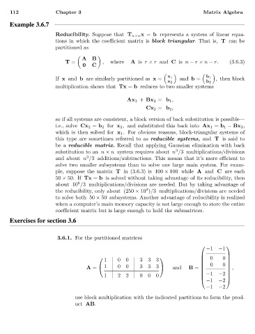
3.6.1. For the partitioned matrices

−1 −1
 

   0 
1 00 333  0 
 0

 ,
A =  1 00 333  and B =  0 


1 22 000  −1 −2 
−1 −2
 
−1 −2
use block multiplication with the indicated partitions to form the prod-
uct AB.