Page 26 - Matrix Analysis & Applied Linear Algebra

18 Chapter 1 Linear Equations
1.4 TWO-POINT BOUNDARY VALUE PROBLEMS

It was stated previously that linear systems that arise in practice can become
quite large in size. The purpose of this section is to understand why this often
occurs and why there is frequently a special structure to the linear systems that
come from practical applications.
Given an interval [a, b] and two numbers α and β, consider the general
problem of trying to find a function y(t) that satisfies the differential equation

u(t)y (t)+v(t)y (t)+w(t)y(t)= f(t), where y(a)= α and y(b)= β. (1.4.1)
The functions u, v, w, and f are assumed to be known functions on [a, b].
Because the unknown function y(t) is specified at the boundary points a and
b, problem (1.4.1) is known as a two-point boundary value problem. Such
problems abound in nature and are frequently very hard to handle because it is
often not possible to express y(t) in terms of elementary functions. Numerical
methods are usually employed to approximate y(t) at discrete points inside
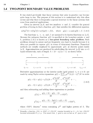
[a, b]. Approximations are produced by subdividing the interval [a, b]into n+1
equal subintervals, each of length h =(b − a)/(n + 1) as shown below.
h h h
···

t 0 = a t 1 = a + h t 2 = a +2h ··· t n = a + nh t n+1 = b
Derivative approximations at the interior nodes (grid points) t i = a + ih are
∞ (k) k
made by using Taylor series expansions y(t)= y (t i )(t−t i ) /k! to write
k=0

y (t i )h 2 y (t i )h 3
y(t i + h)= y(t i )+ y (t i )h + + + ··· ,

2! 3!
(1.4.2)
y (t i )h 2 y (t i )h 3

y(t i − h)= y(t i ) − y (t i )h + − + ··· ,
2! 3!
and then subtracting and adding these expressions to produce
y(t i + h) − y(t i − h) 3
y (t i )= + O(h )

2h
and
y(t i − h) − 2y(t i )+ y(t i + h) 4
y (t i )= + O(h ),

h 2
p
where O(h ) denotes 5 terms containing p th and higher powers of h. The
5
p
Formally,a function f(h)is O(h )if f(h)/h p remains bounded as h → 0, but f(h)/h q
becomes unbounded if q> p. This means that f goes to zero as fast as h p goes to zero.