Page 29 - Matrix Analysis & Applied Linear Algebra

1.5 Making Gaussian Elimination Work 21
1.5 MAKING GAUSSIAN ELIMINATION WORK

Now that you understand the basic Gaussian elimination technique, it’s time
to turn it into a practical algorithm that can be used for realistic applications.
For pencil and paper computations where you are doing exact arithmetic, the
strategy is to keep things as simple as possible (like avoiding messy fractions) in
order to minimize those “stupid arithmetic errors” we are all prone to make. But
very few problems in the real world are of the textbook variety, and practical
applications involving linear systems usually demand the use of a computer.
Computers don’t care about messy fractions, and they don’t introduce errors of
the “stupid” variety. Computers produce a more predictable kind of error, called
6
roundoff error, and it’s important to spend a little time up front to understand
this kind of error and its effects on solving linear systems.
Numerical computation in digital computers is performed by approximating
the infinite set of real numbers with a finite set of numbers as described below.

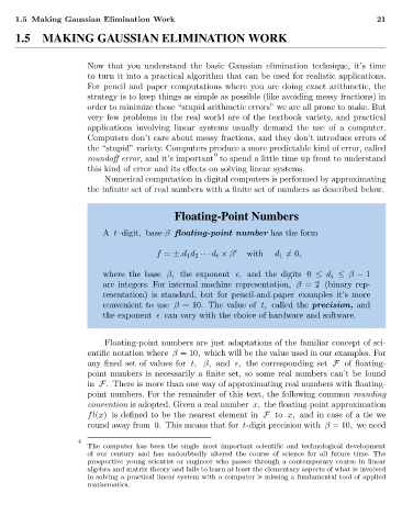
Floating-Point Numbers
A t -digit, base-β floating-point number has the form

f = ±.d 1 d 2 ··· d t × β with d 1 =0,
where the base β, the exponent , and the digits 0 ≤ d i ≤ β − 1
are integers. For internal machine representation, β = 2 (binary rep-
resentation) is standard, but for pencil-and-paper examples it’s more
convenient to use β =10. The value of t, called the precision, and
the exponent can vary with the choice of hardware and software.

Floating-point numbers are just adaptations of the familiar concept of sci-
entific notation where β =10, which will be the value used in our examples. For
any fixed set of values for t, β, and , the corresponding set F of floating-
point numbers is necessarily a finite set, so some real numbers can’t be found
in F. There is more than one way of approximating real numbers with floating-
point numbers. For the remainder of this text, the following common rounding
convention is adopted. Given a real number x, the floating-point approximation
fl(x) is defined to be the nearest element in F to x, and in case of a tie we
round away from 0. This means that for t-digit precision with β =10, we need

6
The computer has been the single most important scientific and technological development
of our century and has undoubtedly altered the course of science for all future time. The
prospective young scientist or engineer who passes through a contemporary course in linear
algebra and matrix theory and fails to learn at least the elementary aspects of what is involved
in solving a practical linear system with a computer is missing a fundamental tool of applied
mathematics.