Page 34 - Matrix Analysis & Applied Linear Algebra

26 Chapter 1 Linear Equations

which is quite different from the original system. With partial pivoting the mul-
tiplier is 10 −4 , and this is small enough so that it does not swamp the numbers
1 and 2. In this case, the 3-digit computer produces the exact solution to the
0 1 1 7
system , which is close to the original system.
1 1 2
In summary, the villain in Example 1.5.1 is the large multiplier that pre-
vents some smaller numbers from being fully accounted for, thereby resulting
in the exact solution of another system that is very different from the original
system. By maximizing the magnitude of the pivot at each step, we minimize
the magnitude of the associated multiplier thus helping to control the growth
of numbers that emerge during the elimination process. This in turn helps cir-
cumvent some of the effects of roundoff error. The problem of growth in the
elimination procedure is more deeply analyzed on p. 348.
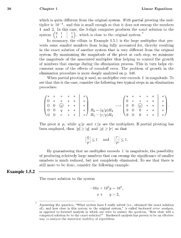
When partial pivoting is used, no multiplier ever exceeds 1 in magnitude. To
see that this is the case, consider the following two typical steps in an elimination
procedure:

   
∗ ∗ ∗ ∗ ∗ ∗ ∗ ∗ ∗ ∗ ∗ ∗
 0 ∗ ∗ ∗ ∗ ∗   0 ∗ ∗ ∗ ∗ ∗ 
   
p
p
 00 ∗∗ ∗  −→  00 ∗∗ ∗  .
00 q ∗∗ ∗ R 4 − (q/p)R 3 00 0 ∗∗ ∗
   
00 r ∗∗ ∗ R 5 − (r/p)R 3 00 0 ∗∗ ∗
The pivot is p, while q/p and r/p are the multipliers. If partial pivoting has
been employed, then |p|≥|q| and |p|≥|r| so that

q r
≤ 1 and ≤ 1.
p p
By guaranteeing that no multiplier exceeds 1 in magnitude, the possibility
of producing relatively large numbers that can swamp the significance of smaller
numbers is much reduced, but not completely eliminated. To see that there is
still more to be done, consider the following example.
Example 1.5.2
The exact solution to the system

5
5
−10x +10 y =10 ,
x + y =2,
7
Answering the question,“What system have I really solved (i.e.,obtained the exact solution
of),and how close is this system to the original system,” is called backward error analysis,
as opposed to forward analysis in which one tries to answer the question,“How close will a
computed solution be to the exact solution?” Backward analysis has proven to be an effective
way to analyze the numerical stability of algorithms.