Page 35 - Matrix Analysis & Applied Linear Algebra

1.5 Making Gaussian Elimination Work 27

is given by
1 1.0002
x = and y = .
1.0001 1.0001
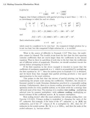
Suppose that 3-digit arithmetic with partial pivoting is used. Since |− 10| > 1,
no interchange is called for and we obtain

5 5 5 5
−10 10 10 −10 10 10
1 1 2 R 2 +10 −1 R 1 −→ 010 4 10 4
because
5
4
5
fl(1+10 )= fl(.10001 × 10 )= .100 × 10 =10 4
and
4
5
4
5
fl(2+10 )= fl(.10002 × 10 )= .100 × 10 =10 .
Back substitution yields
x = 0 and y =1,
which must be considered to be very bad—the computed 3-digit solution for y
is not too bad, but the computed 3-digit solution for x is terrible!
What is the source of difficulty in Example 1.5.2? This time, the multi-
plier cannot be blamed. The trouble stems from the fact that the first equation
contains coefficients that are much larger than the coefficients in the second
equation. That is, there is a problem of scale due to the fact that the coefficients
are of different orders of magnitude. Therefore, we should somehow rescale the
system before attempting to solve it.
If the first equation in the above example is rescaled to insure that the
coefficient of maximum magnitude is a 1, which is accomplished by multiplying
the first equation by 10 −5 , then the system given in Example 1.5.1 is obtained,
and we know from that example that partial pivoting produces a very good
approximation to the exact solution.
This points to the fact that the success of partial pivoting can hinge on
maintaining the proper scale among the coefficients. Therefore, the second re-
finement needed to make Gaussian elimination practical is a reasonable scaling
strategy. Unfortunately, there is no known scaling procedure that will produce
optimum results for every possible system, so we must settle for a strategy that
will work most of the time. The strategy is to combine row scaling—multiplying
selected rows by nonzero multipliers—with column scaling—multiplying se-
lected columns of the coefficient matrix A by nonzero multipliers.
Row scaling doesn’t alter the exact solution, but column scaling does—see
Exercise 1.2.13(b). Column scaling is equivalent to changing the units of the
k th unknown. For example, if the units of the k th unknown x k in [A|b] are
millimeters, and if the k th column of A is multiplied by . 001, then the k th
ˆ
unknown in the scaled system [A | b]is ˆx i = 1000x i , and thus the units of the
scaled unknown ˆx k become meters.