Page 33 - Matrix Analysis & Applied Linear Algebra

1.5 Making Gaussian Elimination Work 25

−4 −4
−10 1 1 −10 1 1
4
1 1 2 R 2 +10 R 1 −→ 0 10 4 10 4
because
4
5
5
fl(1+10 )= fl(.10001 × 10 )= .100 × 10 =10 4 (1.5.1)
and
5
4
4
5
fl(2+10 )= fl(.10002 × 10 )= .100 × 10 =10 . (1.5.2)
Back substitution now produces
x = 0 and y =1.
Although the computed solution for y is close to the exact solution for y, the
computed solution for x is not very close to the exact solution for x —the
computed solution for x is certainly not accurate to three significant figures as
you might hope. If 3-digit arithmetic with partial pivoting is used, then the result
is
−4
−10 1 1 1 1 2
−→ −4 −4
1 1 2 −10 1 1 R 2 +10 R 1

11 2
−→
01 1
because
1
1
fl(1+10 −4 )= fl(.10001 × 10 )= .100 × 10 =1 (1.5.3)
and
1
1
fl(1+2 × 10 −4 )= fl(.10002 × 10 )= .100 × 10 =1. (1.5.4)
This time, back substitution produces the computed solution
x = 1 and y =1,

which is as close to the exact solution as one can reasonably expect—the com-
puted solution agrees with the exact solution to three significant digits.

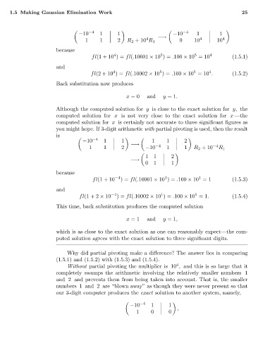
Why did partial pivoting make a difference? The answer lies in comparing
(1.5.1) and (1.5.2) with (1.5.3) and (1.5.4).
4
Without partial pivoting the multiplier is 10 , and this is so large that it
completely swamps the arithmetic involving the relatively smaller numbers 1
and 2 and prevents them from being taken into account. That is, the smaller
numbers 1 and 2 are “blown away” as though they were never present so that
our 3-digit computer produces the exact solution to another system, namely,
−4
−10 1 1
,
1 0 0