Page 27 - Matrix Analysis & Applied Linear Algebra

1.4 Two-Point Boundary Value Problems 19

resulting approximations
y(t i +h) − y(t i −h) y(t i −h) − 2y(t i )+ y(t i +h)

y (t i ) ≈ and y (t i ) ≈ 2 (1.4.3)
2h h
are called centered difference approximations, and they are preferred over
less accurate one-sided approximations such as
y(t i + h) − y(t i ) y(t) − y(t − h)

y (t i ) ≈ or y (t i ) ≈ .
h h
The value h =(b − a)/(n + 1) is called the step size. Smaller step sizes pro-
duce better derivative approximations, so obtaining an accurate solution usually
requires a small step size and a large number of grid points. By evaluating the
centered difference approximations at each grid point and substituting the result
into the original differential equation (1.4.1), a system of n linear equations in
n unknowns is produced in which the unknowns are the values y(t i ). A simple
example can serve to illustrate this point.
Example 1.4.1

Suppose that f(t) is a known function and consider the two-point boundary
value problem

y (t)= f(t)on [0, 1] with y(0) = y(1) = 0.
The goal is to approximate the values of y at n equally spaced grid points
t i interior to [0, 1]. The step size is therefore h =1/(n +1). For the sake of
convenience, let y i = y(t i ) and f i = f(t i ). Use the approximation
y i−1 − 2y i + y i+1

≈ y (t i )= f i
2
h
along with y 0 = 0 and y n+1 = 0 to produce the system of equations
2
−y i−1 +2y i − y i+1 ≈−h f i for i =1, 2,...,n.
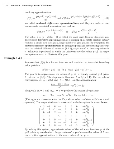
(The signs are chosen to make the 2’s positive to be consistent with later devel-
opments.) The augmented matrix associated with this system is shown below:
2 −1 0 ··· 0 0 0 −h f 1
 2 
2
 −1 2 −1 ··· 0 0 0 −h f 2 
2
 0 −1 2 ··· 0 0 0 −h f 3 


. . . . . . . .
 
 . . . . . . . . . . . . . . . .  .
 
2

 0 0 0 ··· 2 −1 0 −h f n−2 

0 0 0 ··· −1 2 −1 −h f n−1
 2 
2
0 0 0 ··· 0 −1 2 −h f n
By solving this system, approximate values of the unknown function y at the
grid points t i are obtained. Larger values of n produce smaller values of h and
hence better approximations to the exact values of the y i ’s.