
Page 300 - Matrix Analysis & Applied Linear Algebra
P. 300
296 Chapter 5 Norms, Inner Products, and Orthogonality
Example 5.4.2
n
T
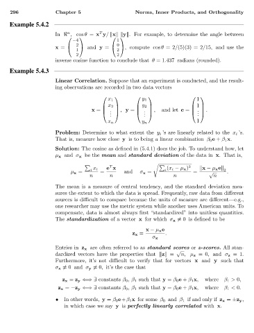
In , cos θ = x y/ x y . For example, to determine the angle between
−4 1
2 0
x = and y = , compute cos θ =2/(5)(3) = 2/15, and use the
1 2
2 2
inverse cosine function to conclude that θ =1.437 radians (rounded).
Example 5.4.3
Linear Correlation. Suppose that an experiment is conducted, and the result-
ing observations are recorded in two data vectors
x 1 y 1 1
x 2 y 2 1
x = . , y = . , and let e = .
.
. . .
. . .
1
x n y n
Problem: Determine to what extent the y i ’s are linearly related to the x i ’s.
That is, measure how close y is to being a linear combination β 0 e + β 1 x.
Solution: The cosine as defined in (5.4.1) does the job. To understand how, let
µ x and σ x be the mean and standard deviation of the data in x. That is,
T (x i − µ x ) 2
µ x = i x i = e x and σ x = i = x − µ x e 2 .
√
n n n n
The mean is a measure of central tendency, and the standard deviation mea-
sures the extent to which the data is spread. Frequently, raw data from different
sources is difficult to compare because the units of measure are different—e.g.,
one researcher may use the metric system while another uses American units. To
compensate, data is almost always first “standardized” into unitless quantities.
The standardization of a vector x for which σ x =0 is defined to be
x − µ x e
z x = .
σ x
Entries in z x are often referred to as standard scores or z-scores. All stan-
√
dardized vectors have the properties that z = n, µ z =0, and σ z =1.
Furthermore, it’s not difficult to verify that for vectors x and y such that
σ x =0 and σ y =0, it’s the case that
z x = z y ⇐⇒ ∃ constants β 0 ,β 1 such that y = β 0 e + β 1 x, where β 1 > 0,
z x = −z y ⇐⇒ ∃ constants β 0 ,β 1 such that y = β 0 e + β 1 x, where β 1 < 0.
• In other words, y = β 0 e+β 1 x for some β 0 and β 1 if and only if z x = ±z y ,
in which case we say y is perfectly linearly correlated with x.